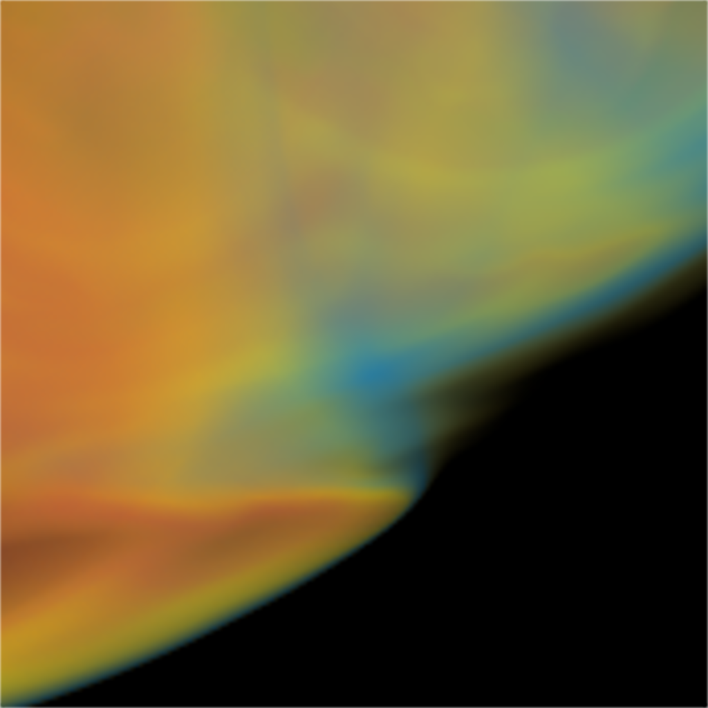
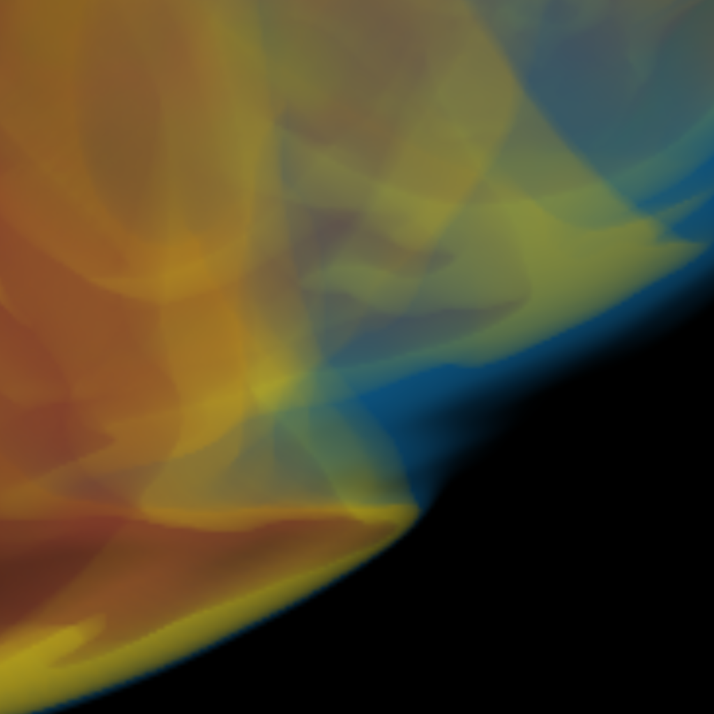
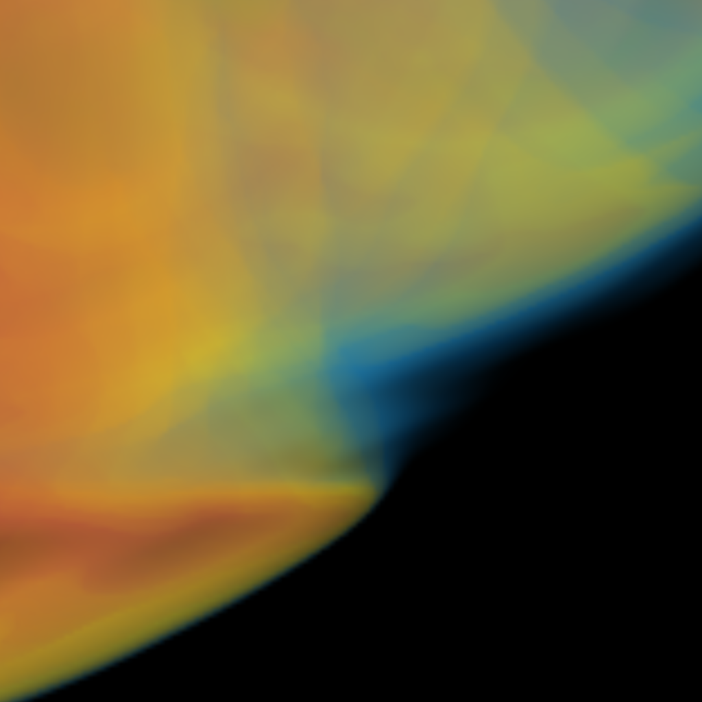
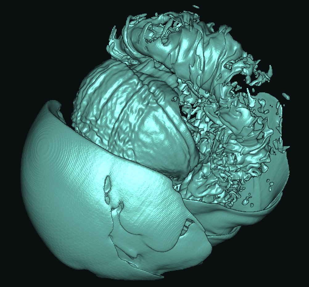
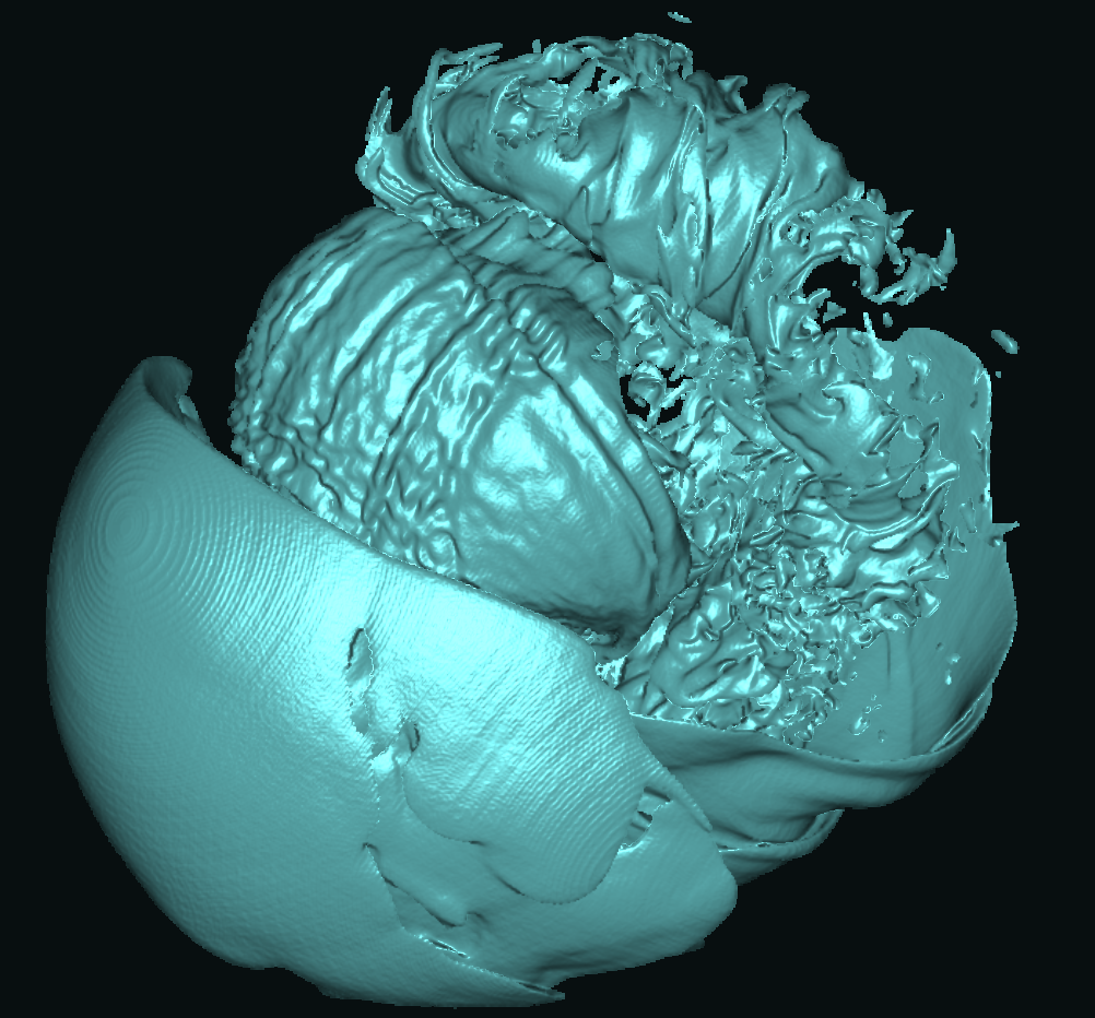
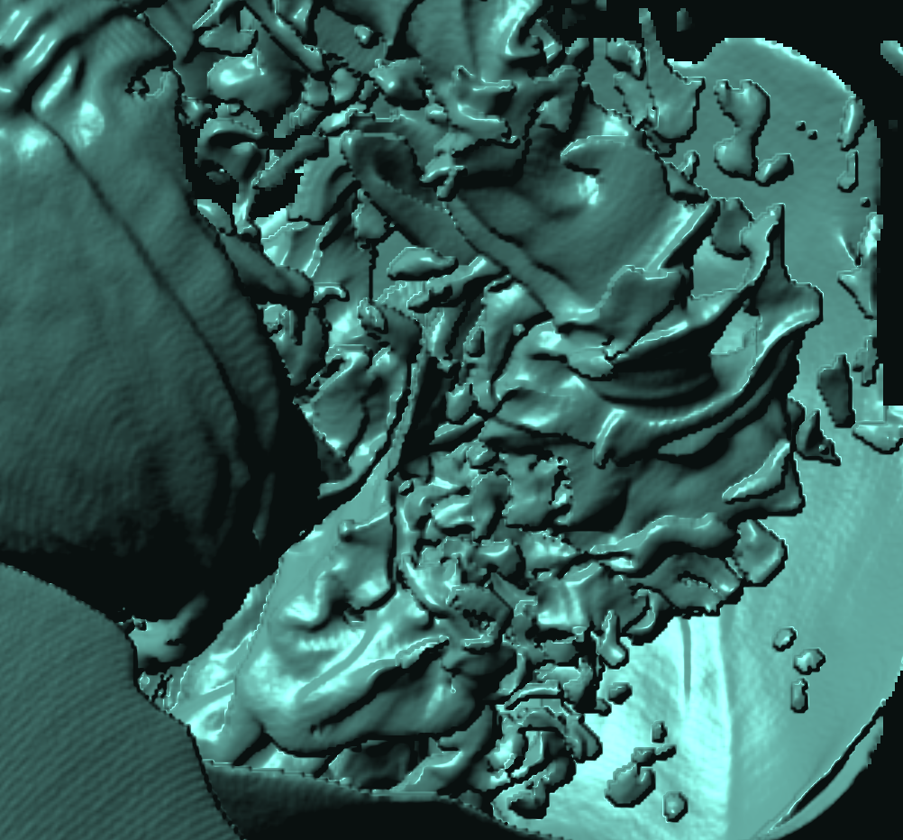
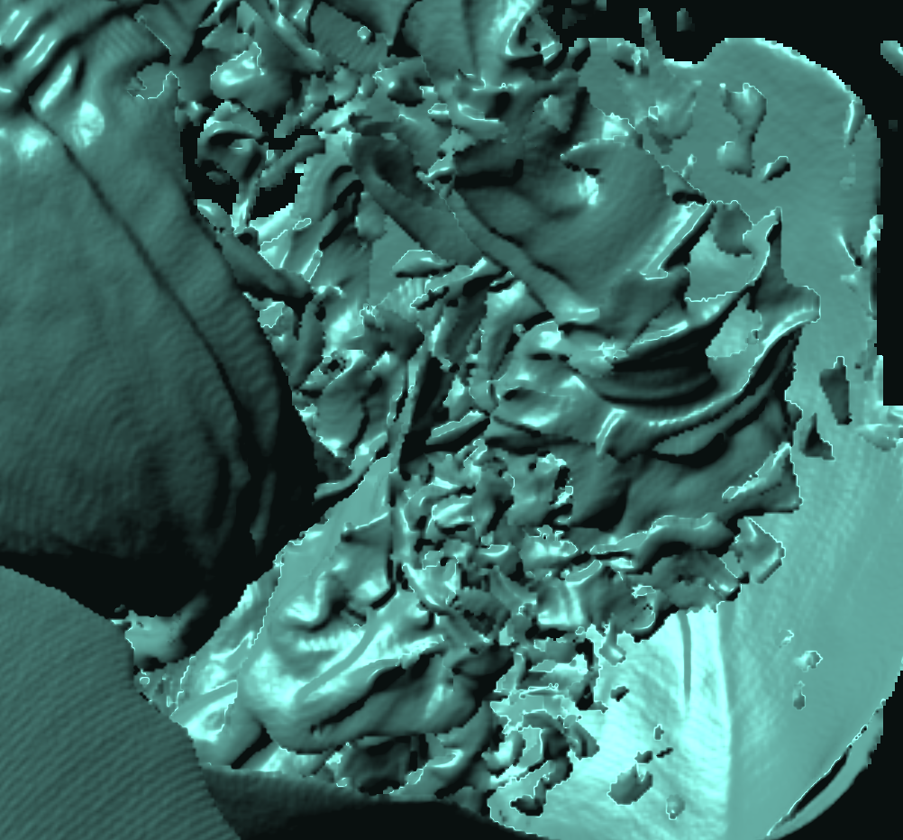
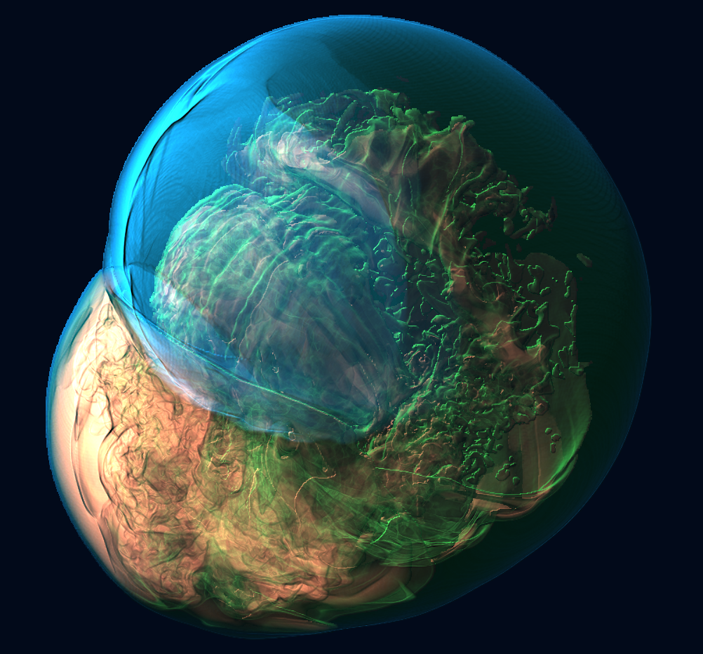
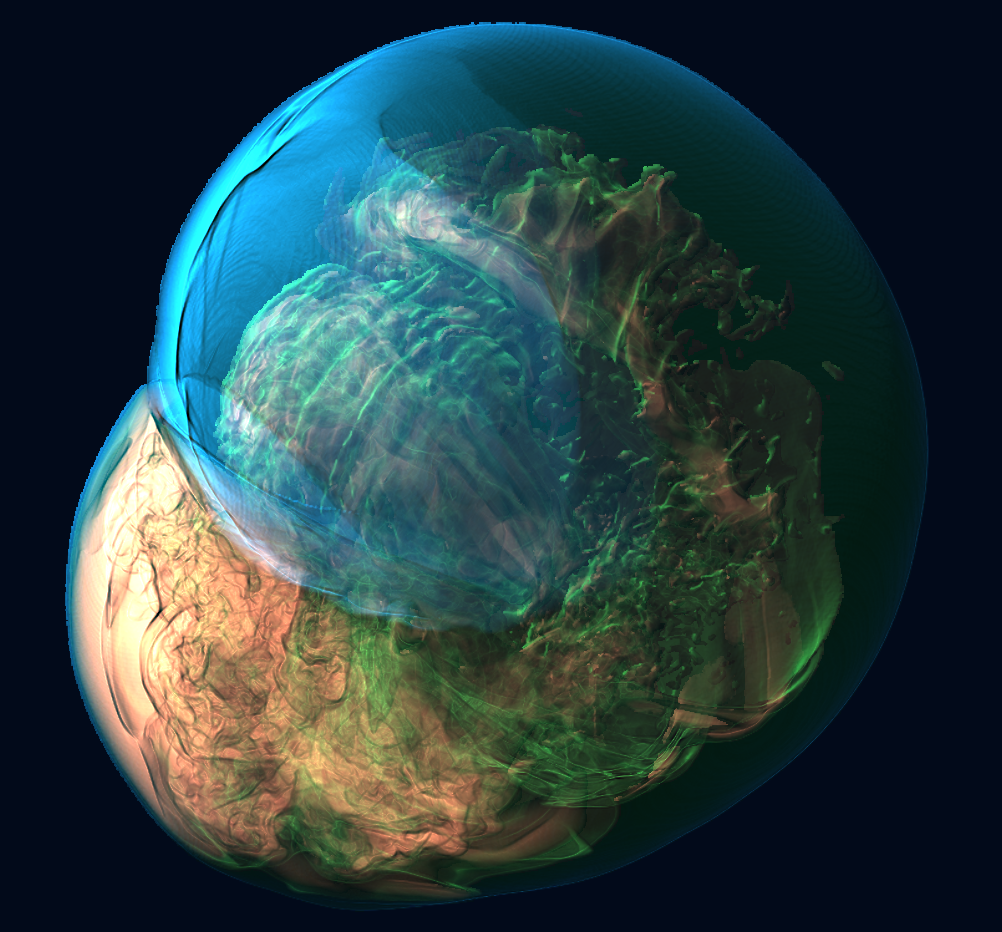
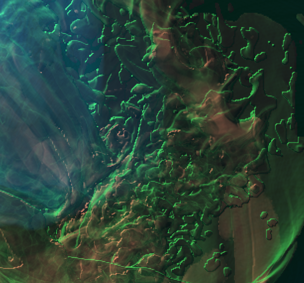
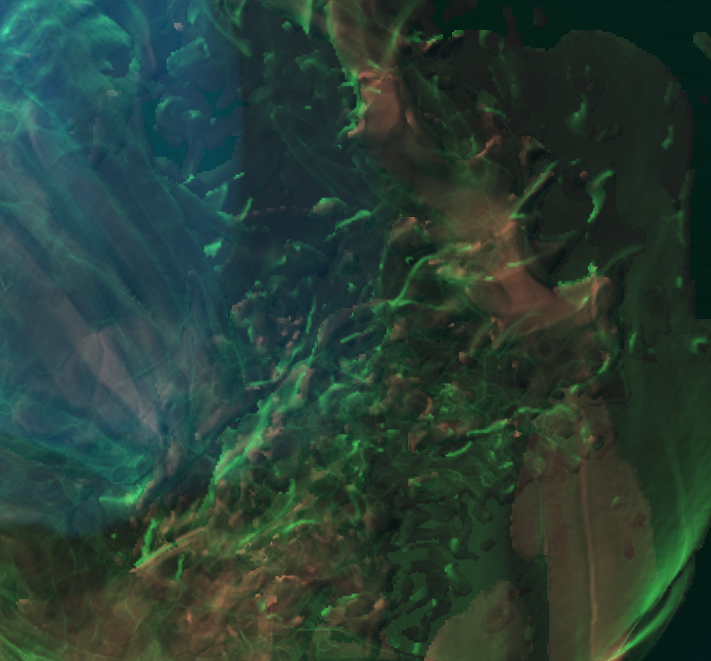
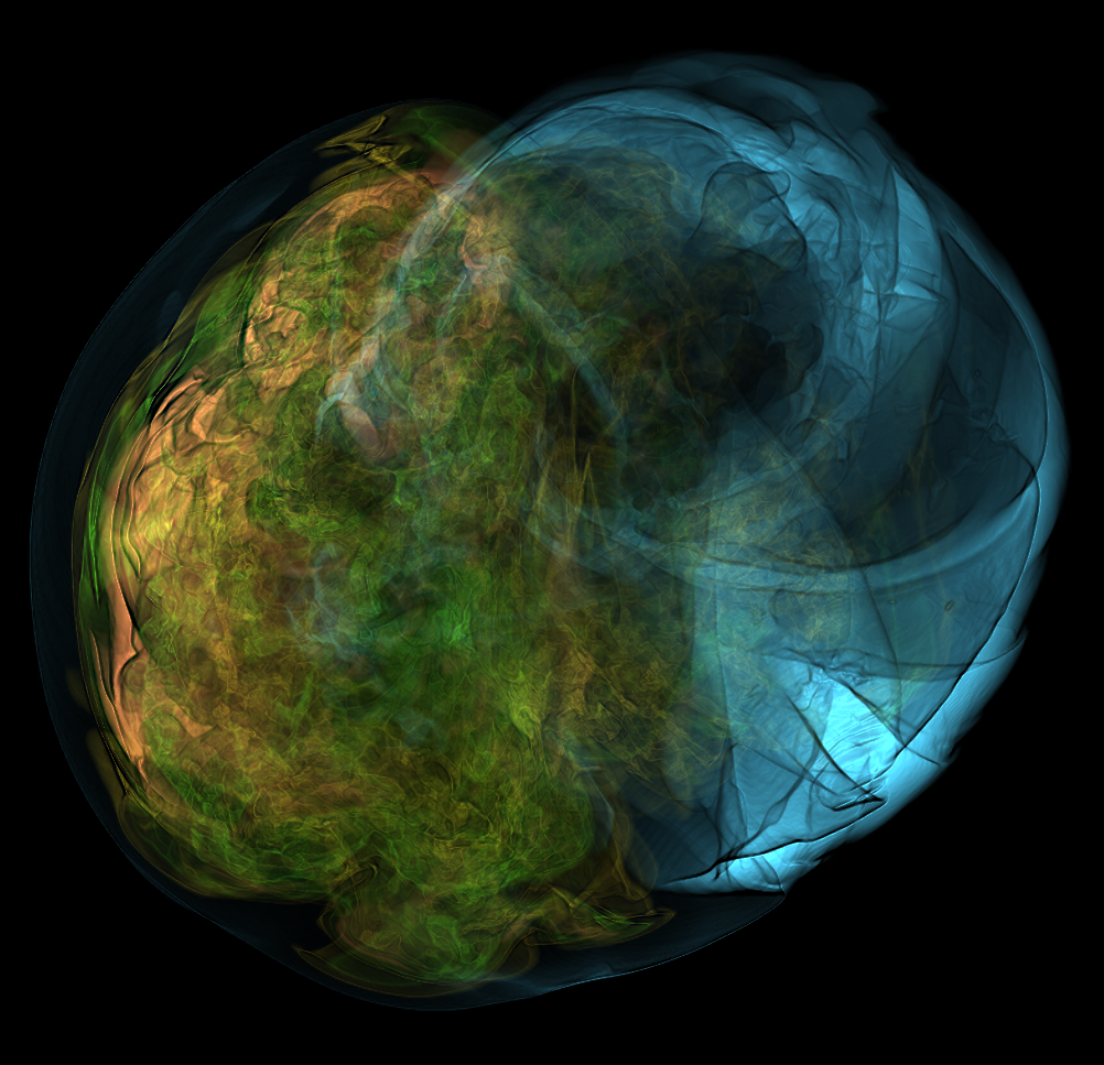
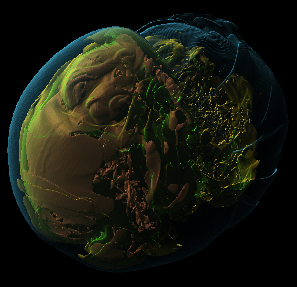
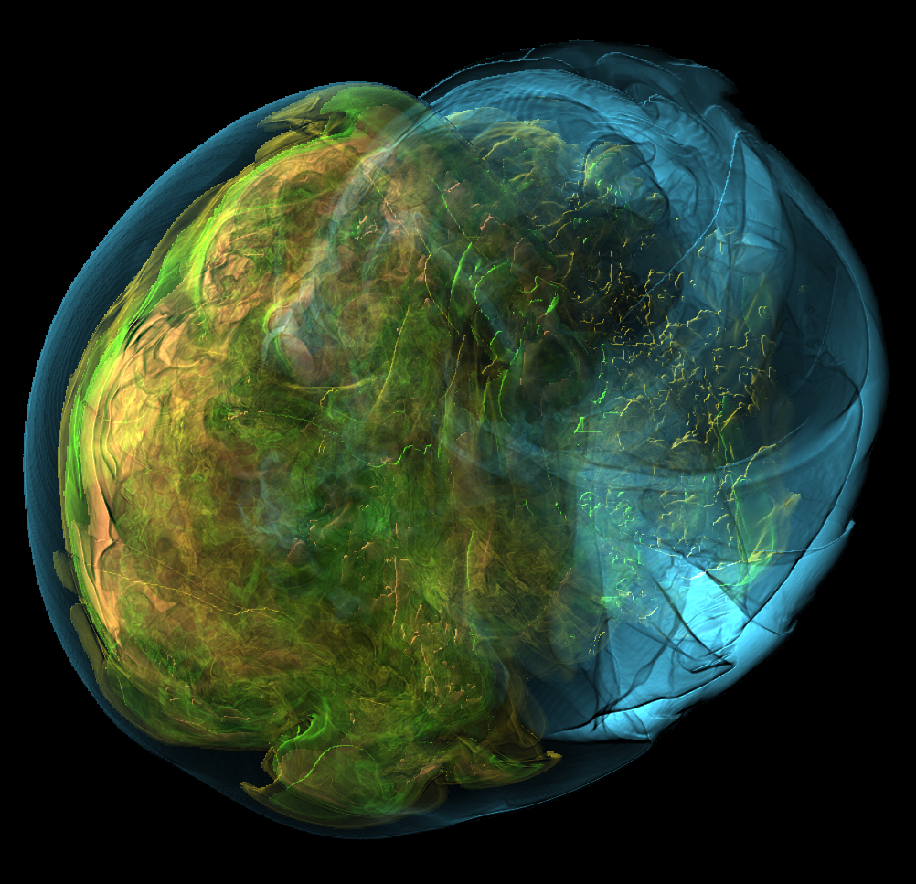
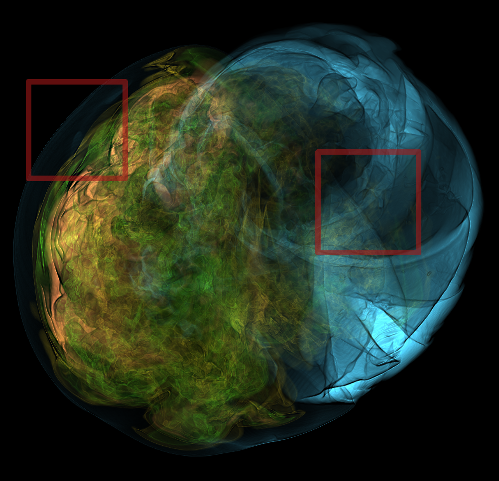
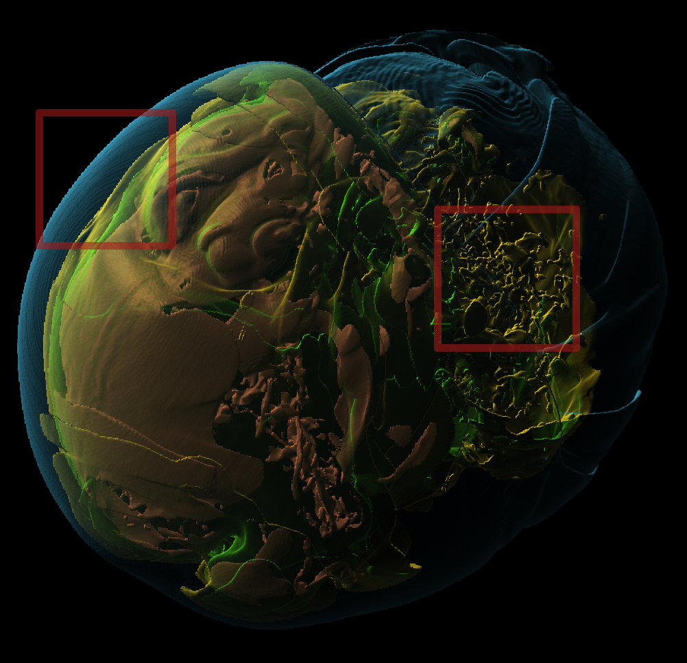
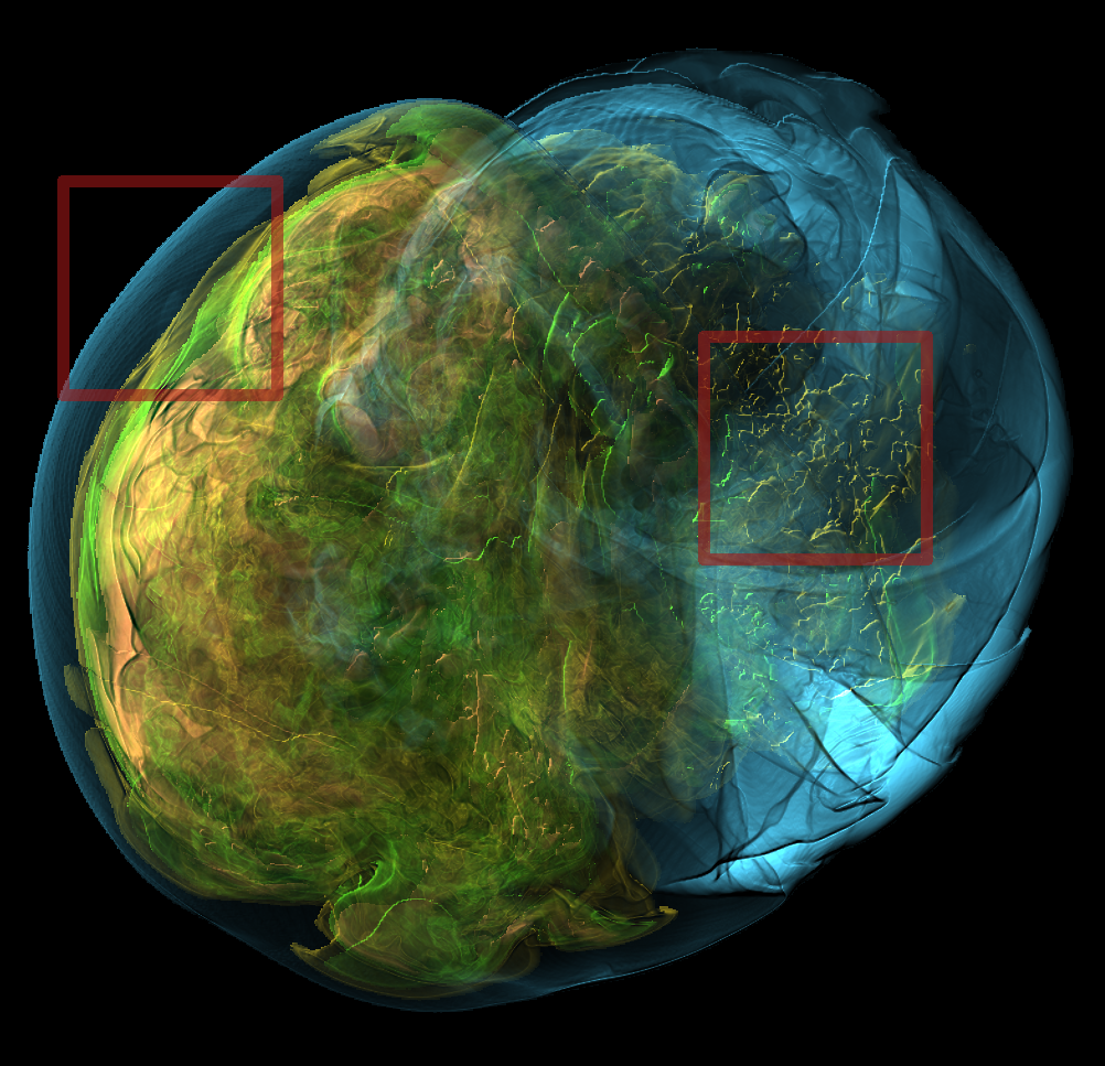
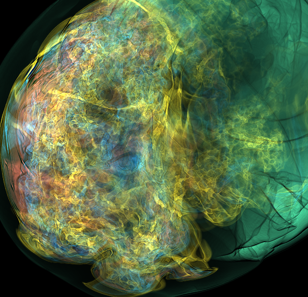
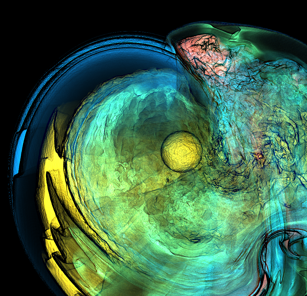
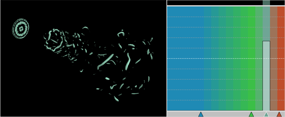
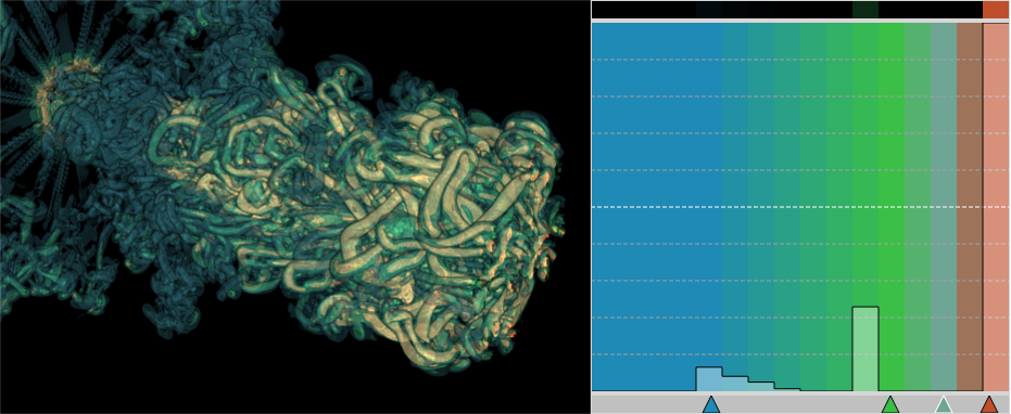
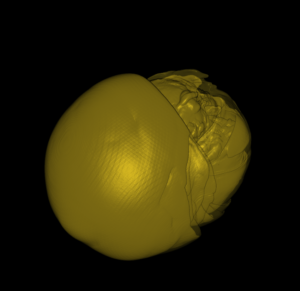
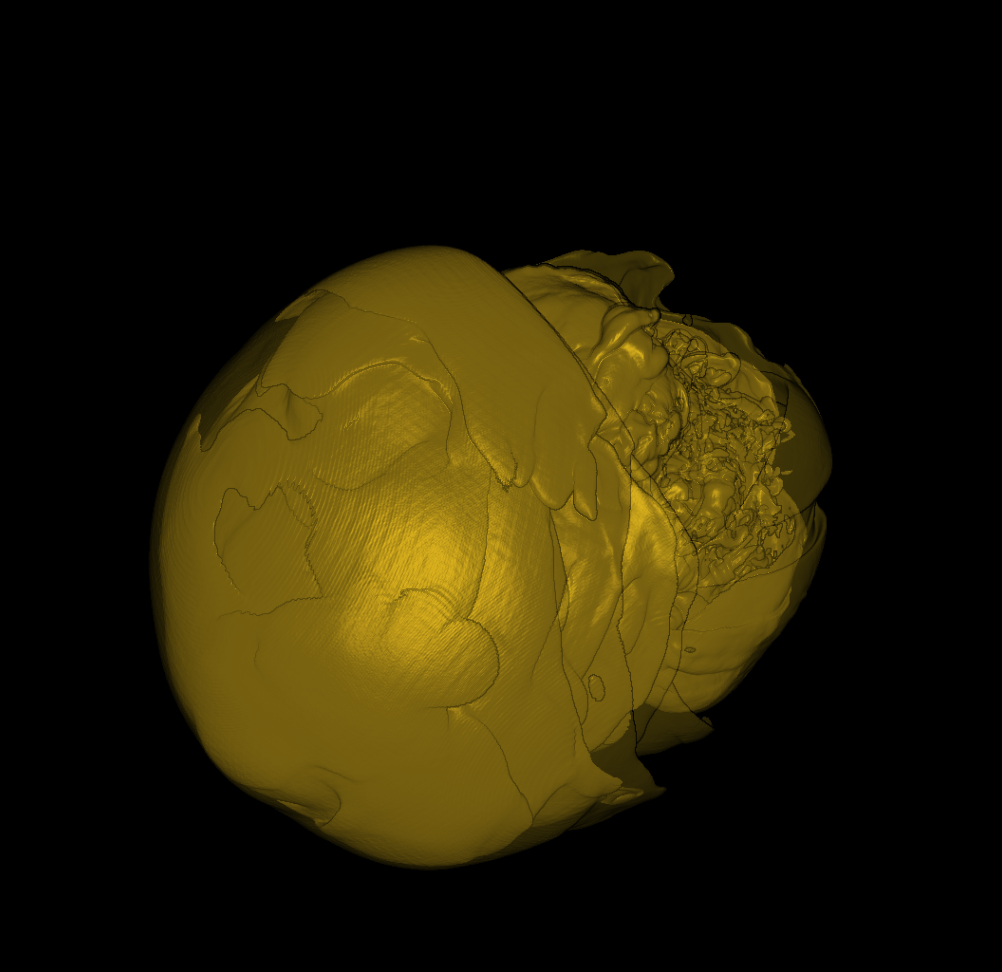
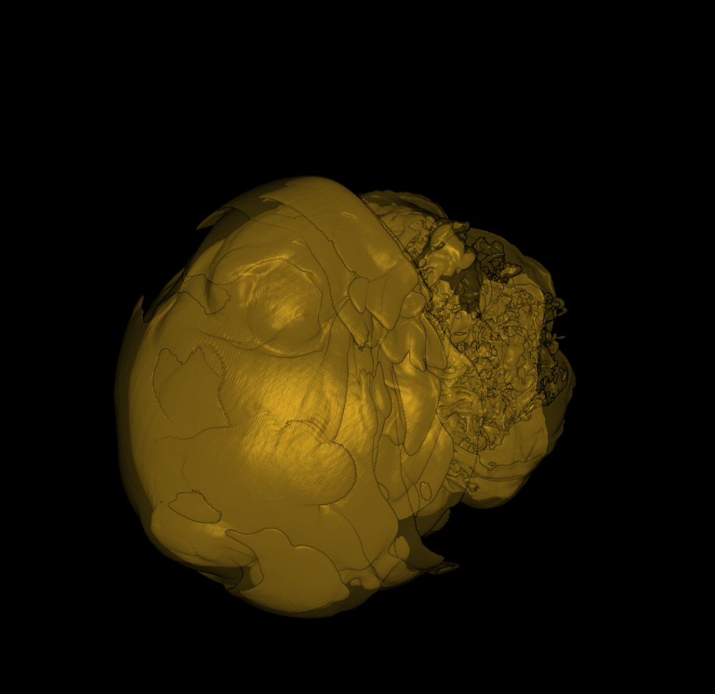
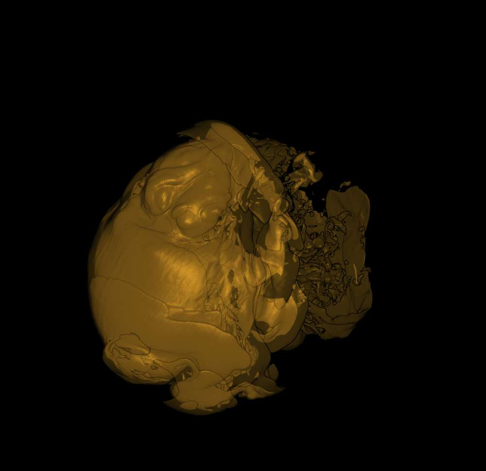
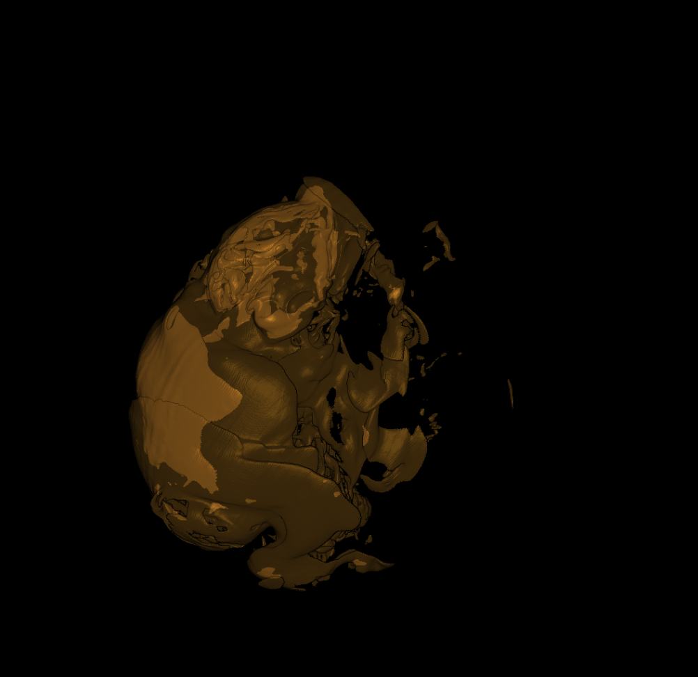
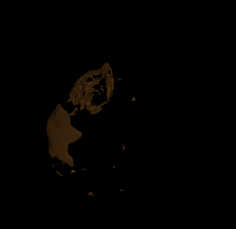
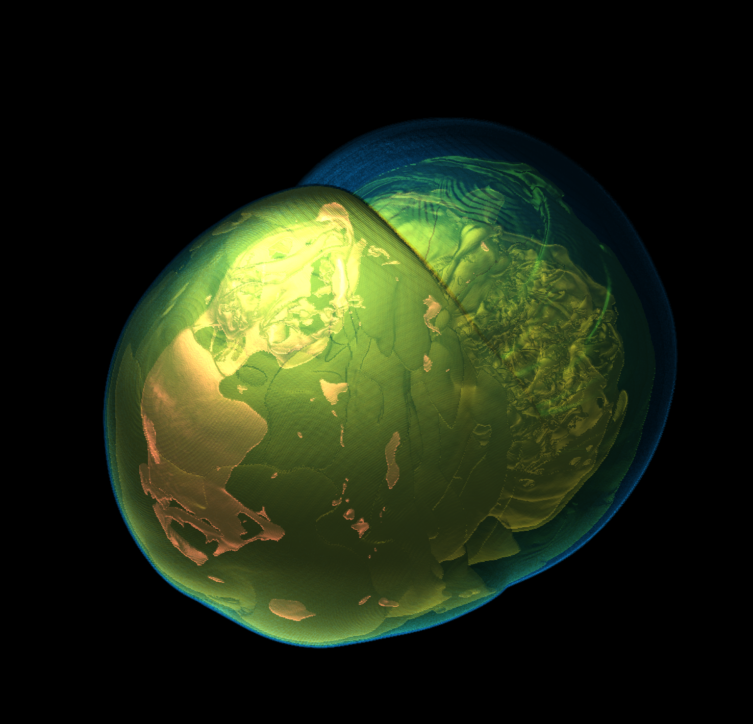
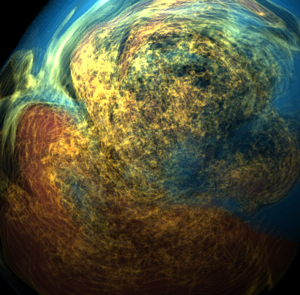
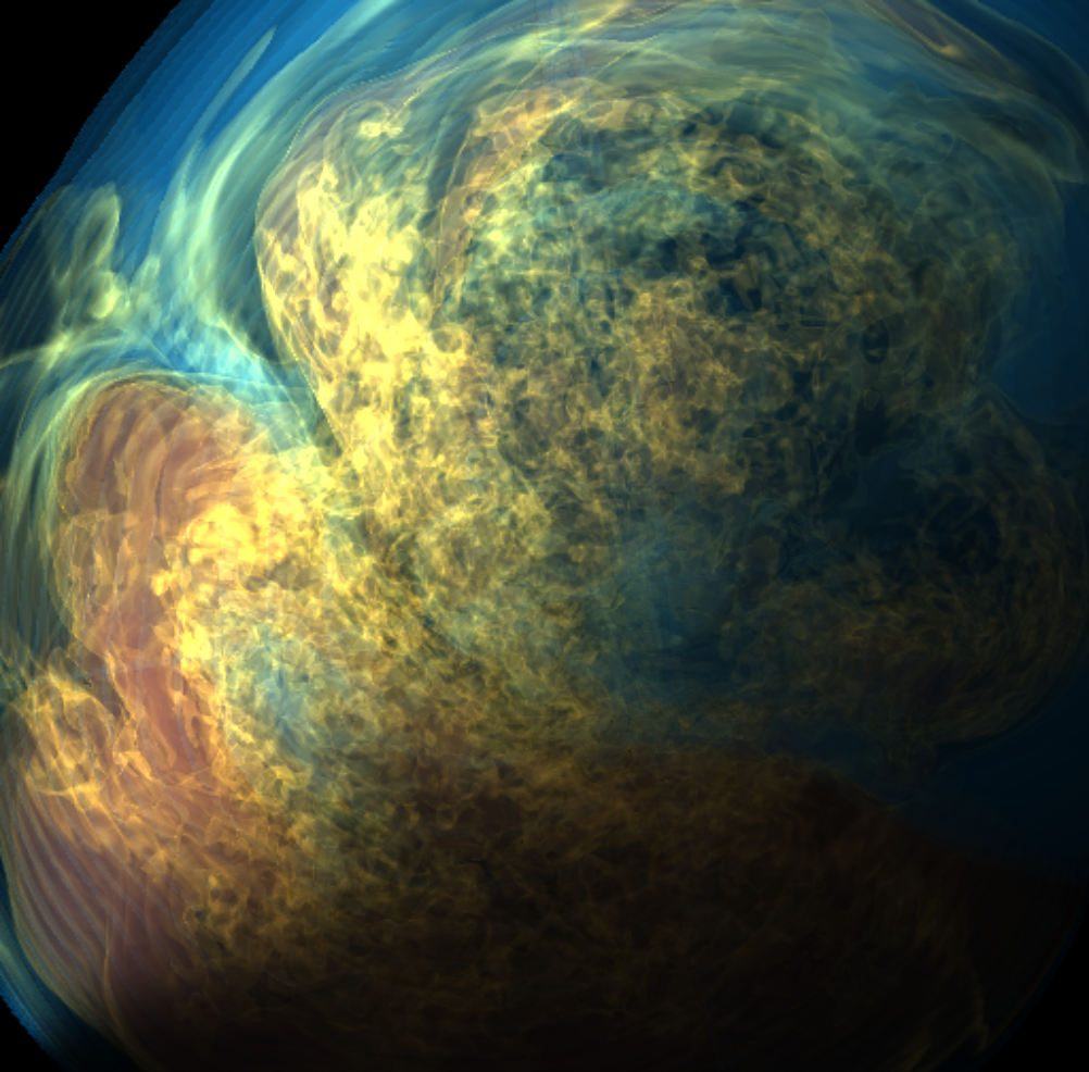
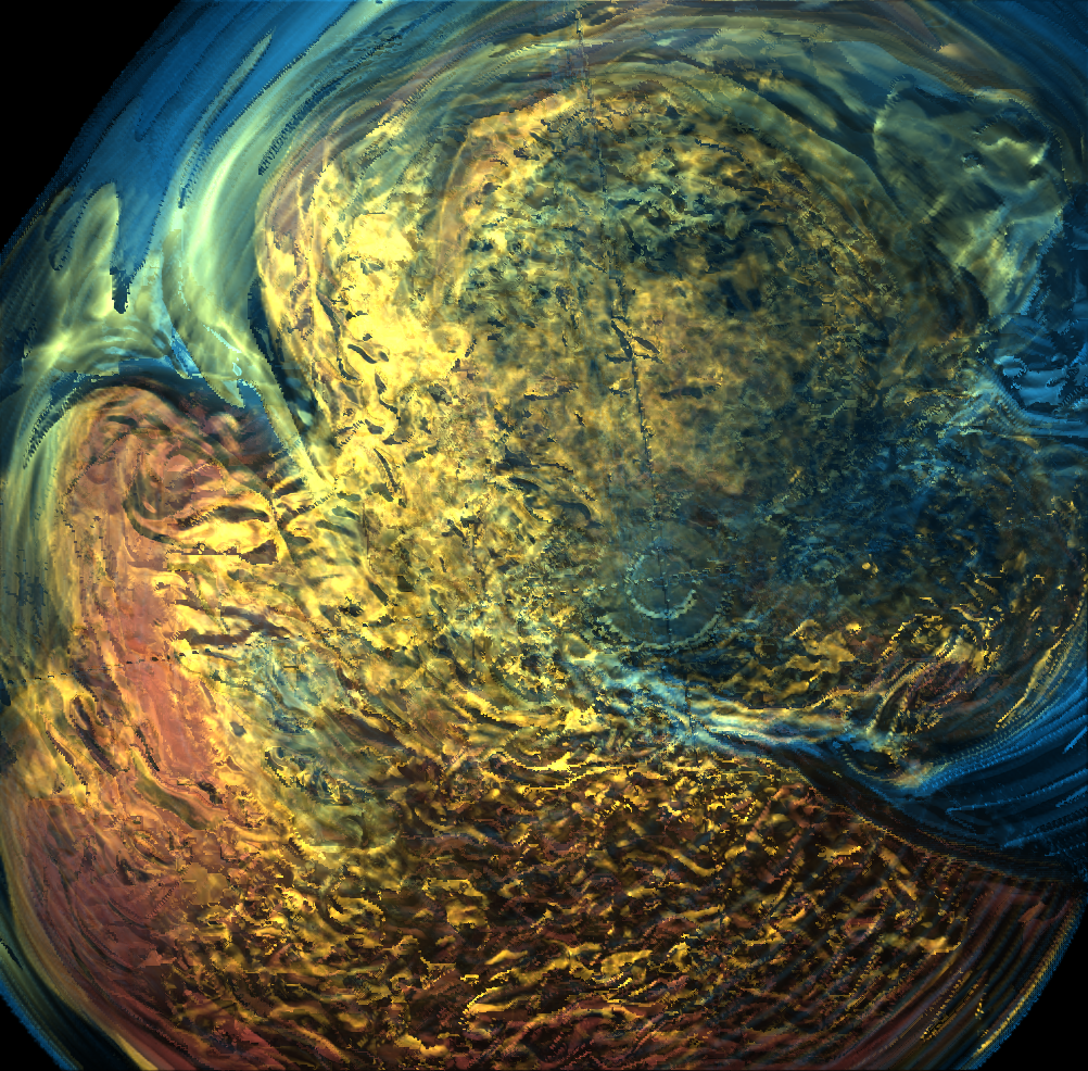
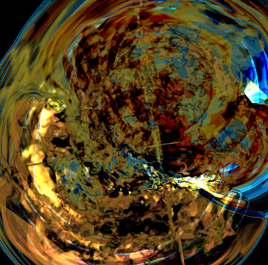
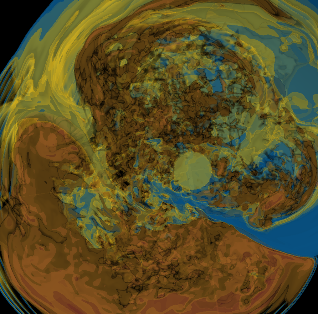
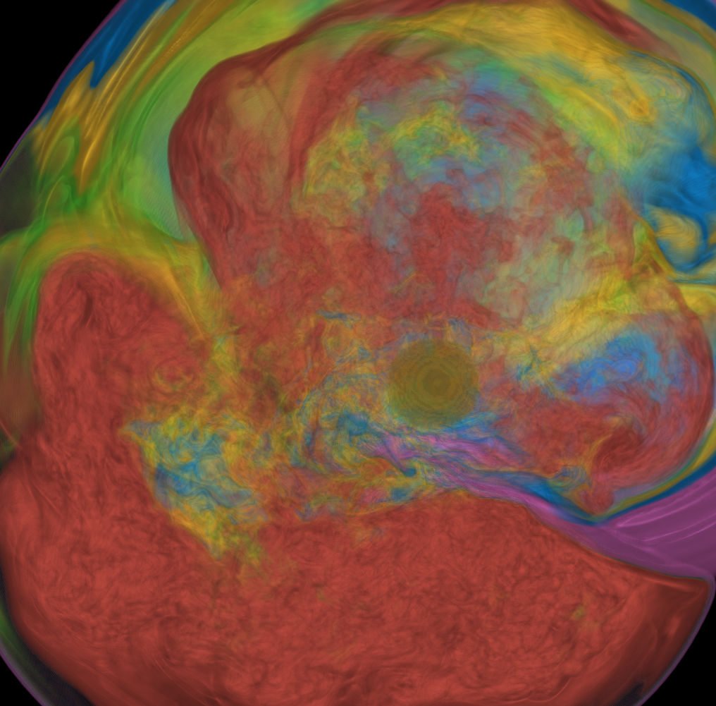
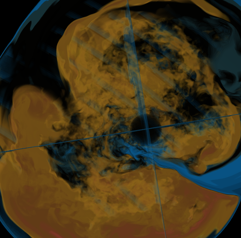
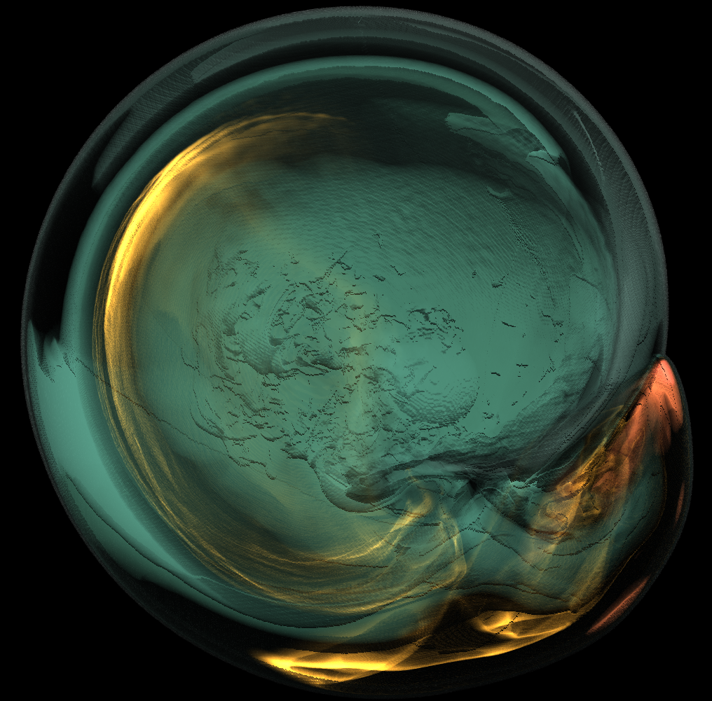
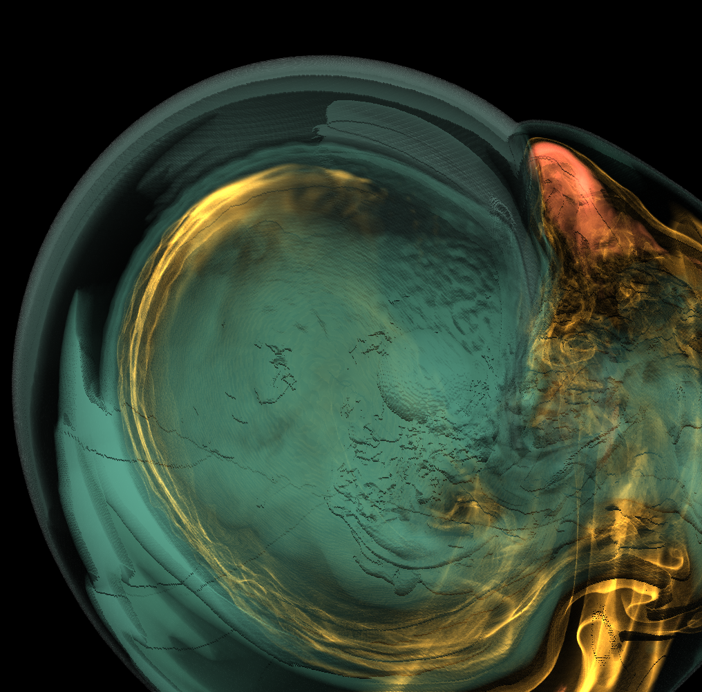
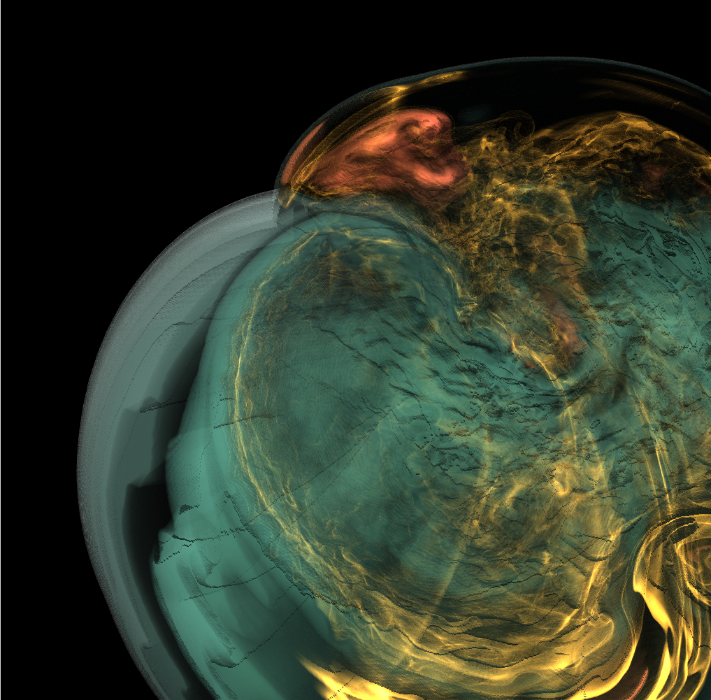
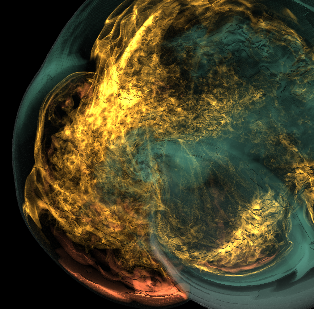
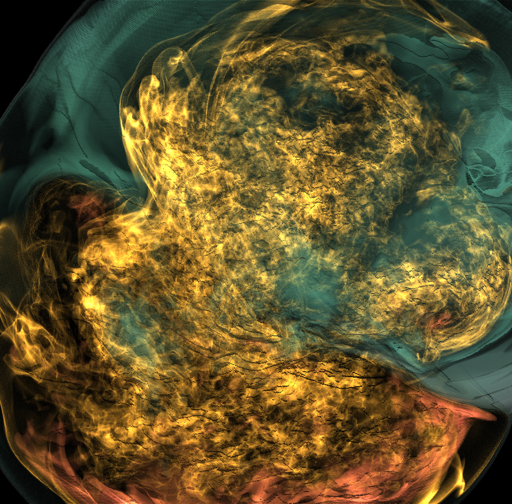
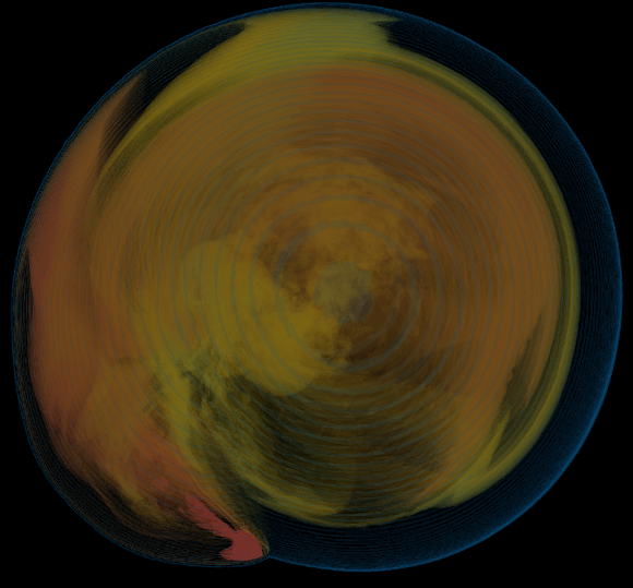
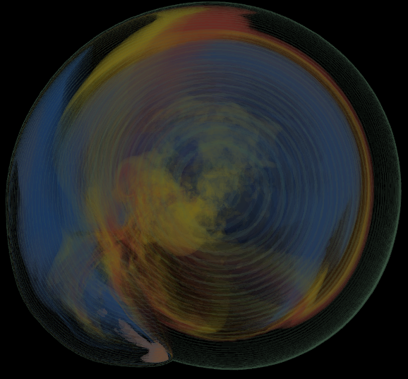
Basically, I finally am able to generate explorable images with different number of bins. These 3 images are the same zoom in spot as the last post. We can see the image is smoother with 32 bins than 16 bins, but less smooth than the ground truth. (As expected).
But, we can generate explorable images with different number of bins now! Some clean up of the codes might be necessary but the functionality is there.
Using Smooth Transfer Function Sep. 4th
This comparison shows the weakness of explorable image because of the small number of bins. The ground truth images are generated using a high resolution (1024) transfer function with linear interpolation enabled. Although the explorable images are generated using the same transfer function, the attenuation values are discretized into a small amount (16) of bins. As a result, the color and opacity changes are more smooth in the ground truth images rather than the images generated from explorable images. We can see the smoothness difference clearly from the zoomed in images.
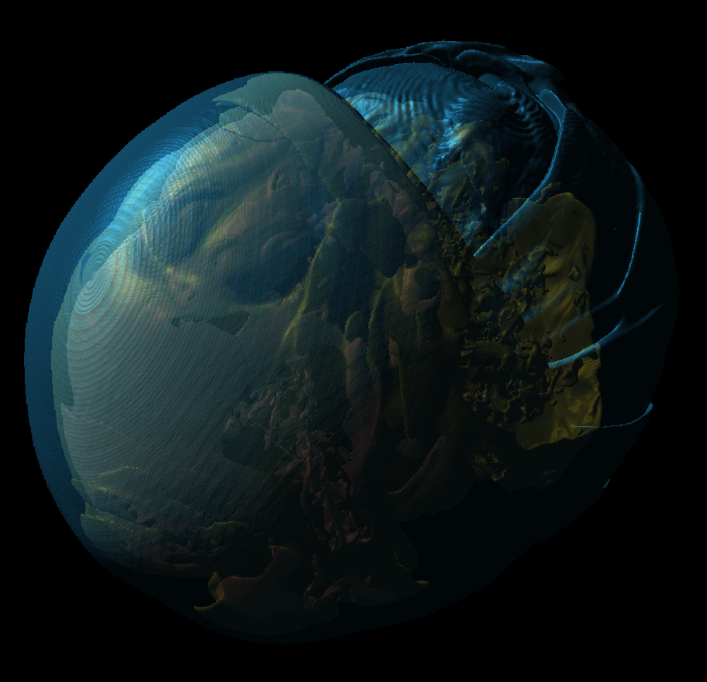
Using Step-function Style Transfer Function August 28th
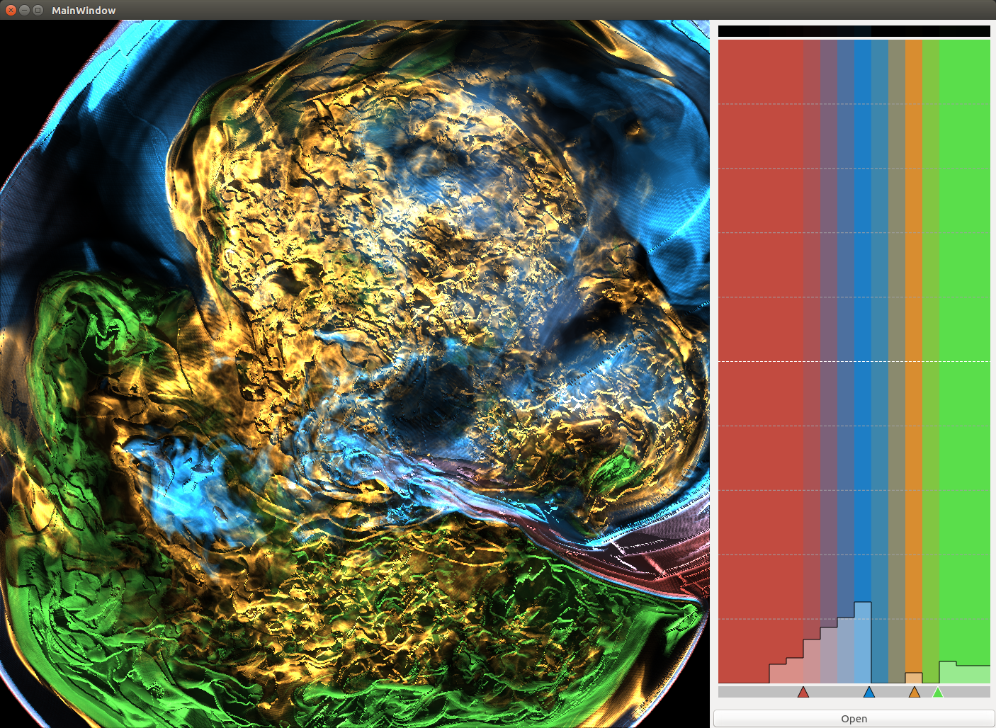
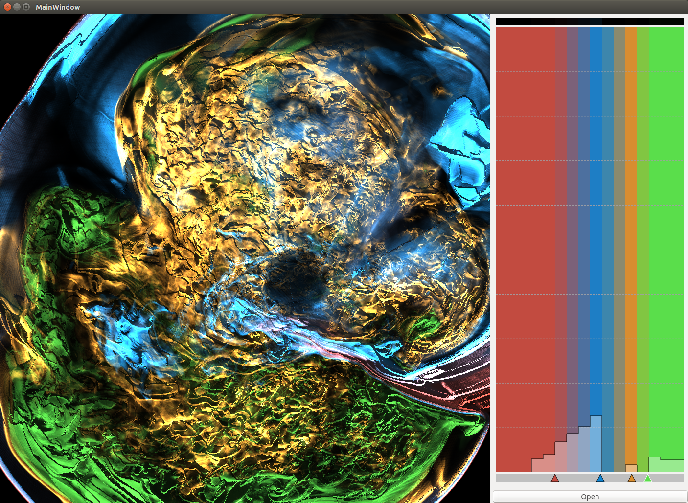
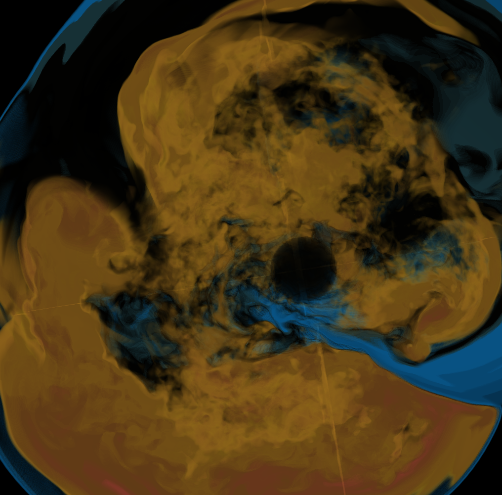
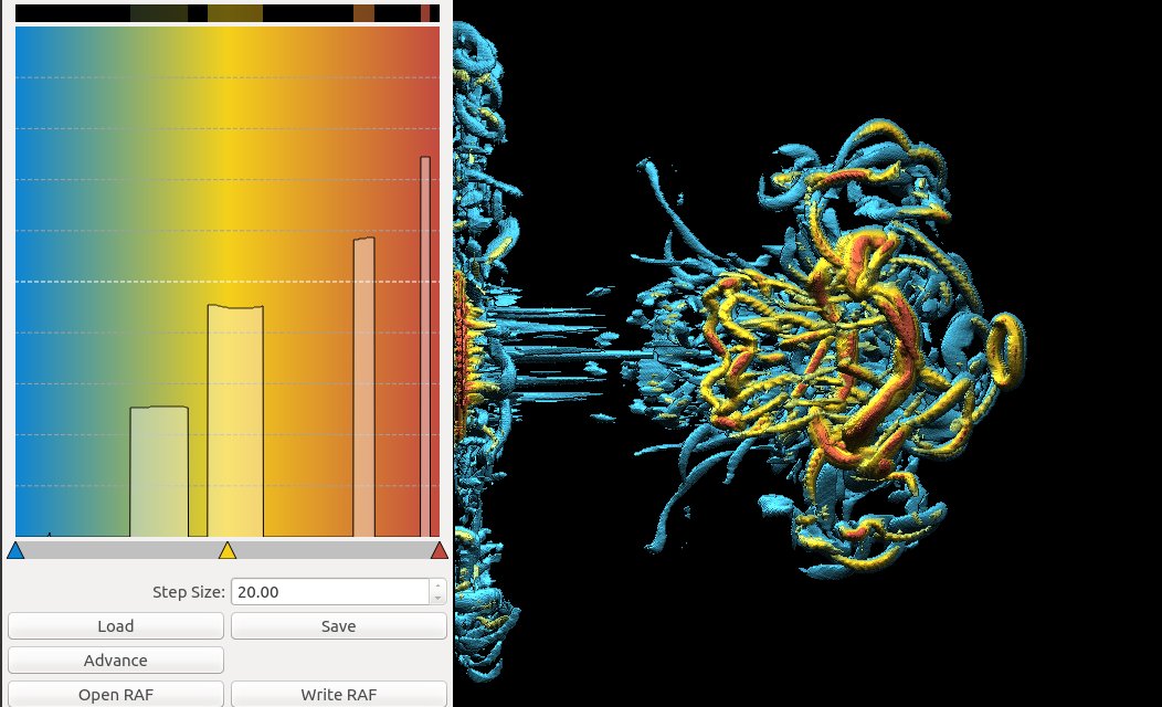
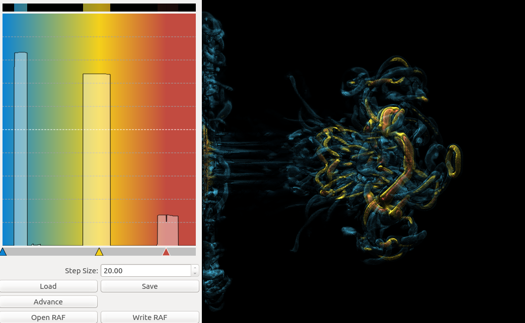
The purpose of this comparison is to analyze how transfer function affects uncertainty. Even though we provide the same transfer function to generate both the volume rendering image and the explorable image, the resulting images can be different because the explorable image reduces the transfer function resolution to number of bins.
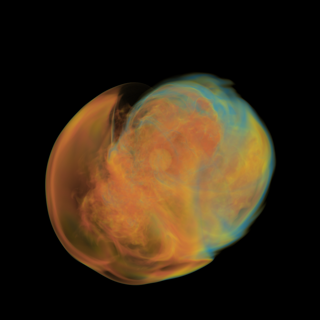
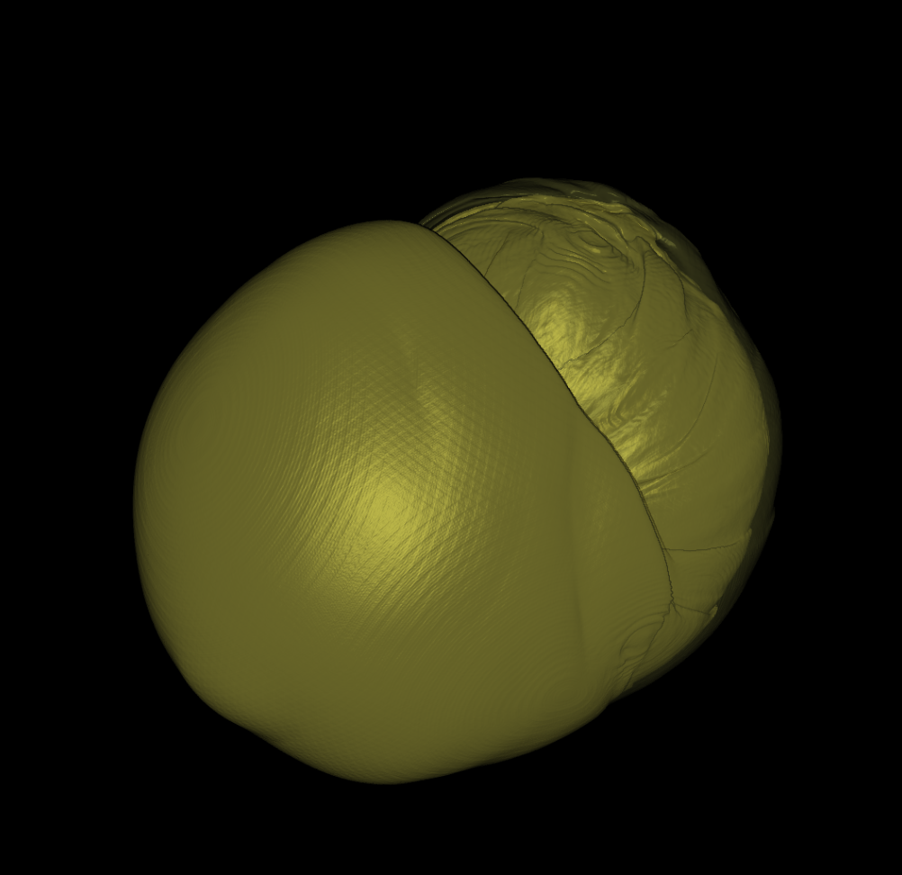
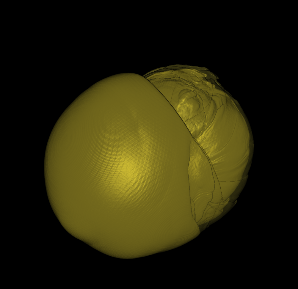
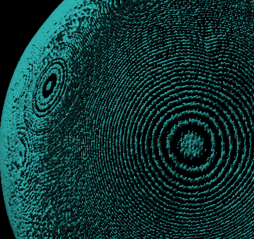
In this comparison, we want to create identical images from both volume rendering and explorable image, and we want to first focus in a single bin (minimum transfer function for explorable image). As a result, we are setting the tranfer function of volume rendering to a step function, where only the opacities in the 11th bin are set to 0.25. Therefore, it mimics the behavior of explorable image.
The first image above is the volume rendering image using the step function style transfer function which only shows the 11th bin. The second image is visualized from the explorable image generated using the same transfer function as the volume rendering image. We can see that they are almost identical. From a zoomed in view, we can actually observe that the volume rendering image has more noise. I am not sure about why that happens.
SC14 Visualization Showcase August 19th
Because the LDAV paper was rejected, we decided to create a submission to Super Computing 2014 Visualization Showcase. It was a video submission that demonstrates high performance computing and visuliazation using explorable images. The video was about 2.5 minutes. The video shown above is the final revision. Before the final revision, we have multiple drafts. I also uploaded the drafts to YouTube as unlisted videos, and they can be found with the following links.
Creating an appealing video is definitely a good experience. I had to learn iMovie and VisKit's animation tool in order to finish this video. I also tried Lightworks. It is definitely more advanced than iMovie, but I ended up using iMovie because it has all the features I need. I can tell that I am definitely more interested in making videos than writing papers.
After the video, we are going to improve the paper and submit it to Pacific Vis.
Submitted and Rejected by LDAV 2014 LDAV 5/14 LDAV 5/26
The following were the milestones of the paper.
Explorable Image Renderer
Generate explorable image with Hongfeng's parallel renderer.
Implement Anna's version
Relighting using depth proxy images
Attenuation clustering and model learning
Parallel reading the data from Dr Ono's simulation.
Yang's Feature Tracking
Yang needs the depth proxy images.
Be able to extract features from a single explorable image.
Track features over time.
Explorable Image Viewer
Incorporate depth proxy images to provide lighting.
Provide interface to specify parameters for the parallel renderer.
Provide interface to select feature from explorable image.
Interface design (timeline?)
Write the Paper
We need at least a proof of concept demo before we can write the paper.
Version 0.1 of SC14 Short Paper August 15th
Click the image for the document.
Live on Github... Not anymore :( July 29th
I finally refactored all the codes and reorganized them in a better way. It's now live on github named HPGVis.
The reason to change the name from ExMage to HPGVis is no reason. Right now I am putting the flow field and scalar field into two separate repositories. I think we should put them together into one repository but in a more elegant way, which means they should be one library, and the configuration file is able specify which to generate.
Although it's on github now, I haven't written the documentation, so that's what I am doing now.
Yet Another New Video July 25th
The purpose of this video is for Kwan-Liu's presentation on July 28th.
The video starts with a bad transfer function, goes to an isosurface rendering, then becomes a volume rendering. After that it plays forward in time. At the end of the time sequence, it changes transfer function again, and finally plays backward in time to the initail frame.
JSON as Configuration Format July 23rd
Instead of using binary configuration file, I have changed to use JSON format. The benefit is that users are able to change the configurations easily by any text editors. The format is indicated below:
{
  // format has to be RAF (Ray Attenuation Function) at the moment

  "format" : "RAF",
  // type is the floating number type, use float or double
  "type" : "float",
  // Specifies the data range. If "minmax" is not provided, the system will calculate it automatically.
  "minmax" : [0.0, 0.1],
  "images" : [
    {
      // Adaptive binning is specified here:
      // It's an array of 17 floating point numbers, the first number is always 0.0, and the last number is always 1.0.
      // If "binTicks" is not provided, the system will use a linear spaced array.
      "binTicks" : [0.0, 0.25, 0.5, 0.625, 0.65626,
                    0.6875, 0.71875, 0.75, 0.765625,
                    0.78125, 0.796875, 0.8125, 0.8281,
                    0.84375, 0.859375, 0.875, 1.0],
      // "sampleSpacing" determines how fast the rays move forward.
      "sampleSpacing" : 0.5
    }
  ],
  "view" : {
    // These determines the resolution of the output image. Usually the last two number of "viewport" are the same as "width" and "height".
    "viewport" : [ 0, 0, 1024, 1024 ],
    "width" : 1024,
    "height" : 1024,
    "angle" : 0,
    "scale" : 0,
    // The model, view, and projection matrix to specify the camera orientation.
    "modelview" : [
      -0.5036, 0.6476, -0.5717, 128.3415,
      0.5741, -0.2436, -0.7816, 135.3691,
      -0.6455, -0.7219, -0.2491, -415.0219,
      0, 0, 0, 1
    ],
    "projection" : [
      2.823912858963013, 0, 0, 0,
      0, 2.823912858963013, 0, 0,
      0, 0, -1.649572372436523, -939.01904296875,
      0, 0, -1, 0
    ]
  }
}
This configuration file is used to generate the supernova (600x600x600) explorable images.
New Supernova Video (DAE + ISO) July 17th
This video is generated when we enable both isosurface rendering and depth-aware enhancment. The light is comming from the upper left corner.
Timestep 62, 63, 160, and 161 are generating some artifacts on the lower right of the image. You can spot the artifacts in the video (They flash for a split second). It seems that the files are partially corrupted since the min max values of these 4 timesteps are significantly different than the others.
To generate this video, I had to regenerate the explorable images with a fixed min max range.
Reduced Edge Emphasis July 16th
I finally found the cause of those bright/black edges, so I fixed them. These images show a comparison between before and after fixing the edges. The images on the left column are the "before" images, which is with clear edges. The images on the right column are the "after" images, which are without clear edges. More detailed descriptions are given in the images.
It ends up I need to take the absolute value of the depth difference before comparing it to a constant cutoff value. Without the absolute operator, only one side of the edges were eliminated.
Note that this improvement is only affecting the isosurface rendering. Nothing is changed for the DAE(depth-aware enhancement) rendering.
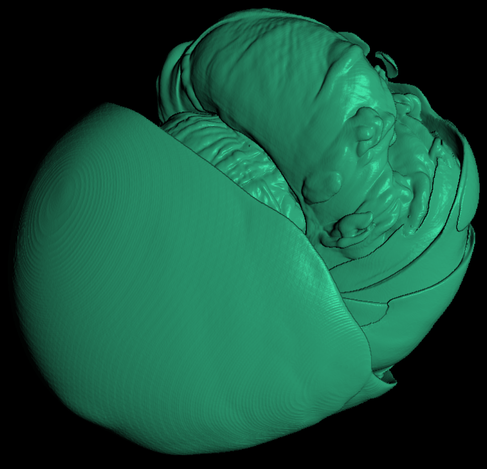
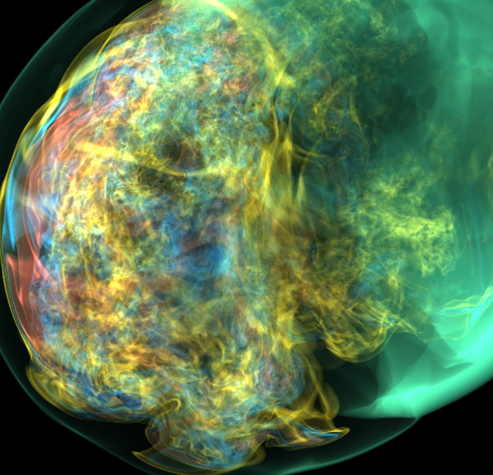
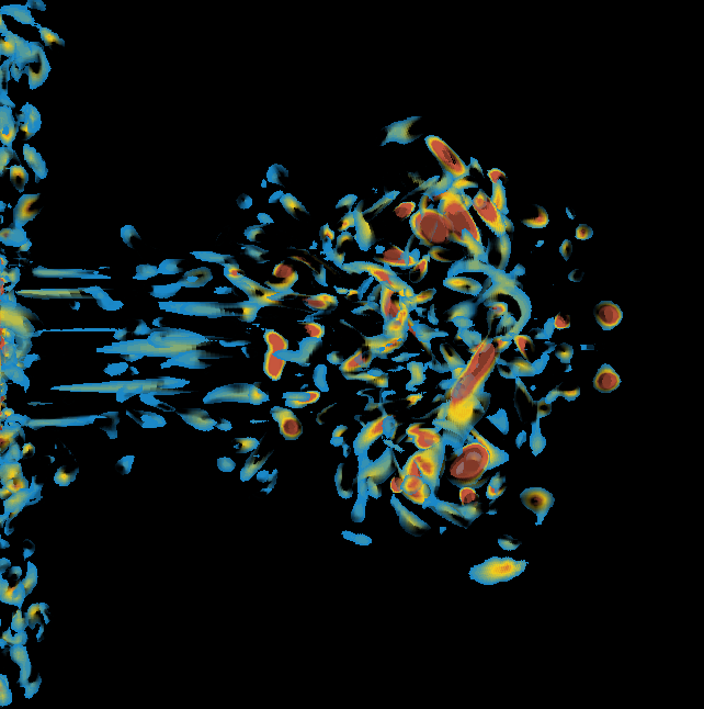
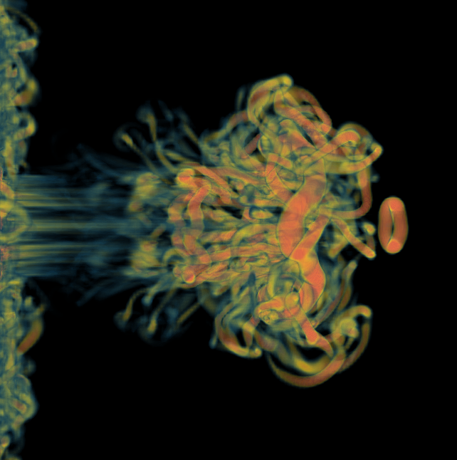
Combining Isosurface and RAF Rendering July 10th
I am trying to combine the RAF rendering (1st image) and the isosurface rendering (2nd image). The results can be seen from the above images. Image 3 is the final result.
I think the results are quite interesting. I won't say it's alot better with it, but it's certainly not worse.
More Translucent Isosurface Rendering July 9th
Previously, the problem with rendering the isosurfaces was that the colors get blended heavily. The result is that the colors of the deeper isosurfaces got altered to the color of the front isosurface. As a result, the colors seem to come from the same color scheme even though they should be completely different.
The way I am approaching this is to alter the opacity based on the normal. When the normal of the pixel is pointing to the camera, we decrease the opacity of the pixel. When the normal of the pixel is orthogonal to the camera, the opacity is higher to indicate there is a surface.
However, some details of the semi transparent isosurfaces can be hidden due to this feature.
The image titles now describe what the image means.
Plan for Lighting June 26th
The tools we have for now: depth-aware enhancement using attenuation gradients and iso surfaces with depth proxy images. The plan is to combine them and provide better lighting.
Depth-aware enhancement is able to highlight the shapes of the features even when they are not the first surface. This enhancement is based on gradients of the attenuation values. The plan is to use these gradients to estimate the normals of these hidden features so that the rendering can react to the direction of lighting.
On the other hand, we have the depth proxy images. Also, for each depth proxy image, we know the intensity value of it. As a result, we essentially have isosurfaces. The plan is to render these depth proxy images the way we render isosurfaces. The point is to keep it separate from the attenuation values.
At the end, we then combine the two approaches above into a single image. The picture will contain semi transparent isosurfaces while the hidden features are highlighted by depth-aware enhancement.
Depth-aware Enhancement June 26th
I found in Anna's TVCG 2010 paper, there is a depth-aware enhancement equation that somehow fakes lighting, so I implemented it. First image is depth unaware and the second image is depth aware...
The depth-aware enhancement uses the 2d gradient of the bin attenuation values to enhance the depth perception but there is no ways to change the lighting parameters such as light directions.
It seems to me that with depth-aware enhancement, it brings out the edges.
I will take a look at whether it is possible to incorporate depth-aware enhancement with the lighting we did using the depth proxy images.
A Cache for Loading Images June 24th
After solving the performance issue of the normal map, the file I/O of the RAF files become the bottleneck. I am trying to use a buffer window to ease the pain of loading files. This will incorporate threading so the other benefit for me is to learn threading.
I choose to go with std::thread instead of Qt tread because std::thread can be used in more places.
Class ImageCache is created for this purpose. In this class we have two std::maps. First maps file index to loaded image, second maps file index to std::thread.
First implementation performs the cache operation when user changes the time slider, but that causes a problem which when user changes the time frequently, it will spawn a lot of threads and that freezes the program. Therefore, we should only allow caching to be perform on idle.
In QSlider, there is a tracking variable. When tracking is true, it means the slider to emit valueChanged on drag. When tracking is false, the slider will only emit valueChanged on mouse release.
The final implementation is to have only 1 extra thread to handle the buffering. When user interacts with the slider, the system delays 1 second before it tries to buffer. The cache operation first deletes the threads outsite of the buffer zone, then load the forward images and finally the backward images.
Some future work can be caching a rendered image so that it can immediately respond to user interaction without any delay, but I am happy with the speed for now.
Faster Normal Map June 19th
The speed of generating normal maps when loading a RAF file is drastically increased.
The normal estimation in the viewer has been a tricky question. At first, we compute the normal in the same pass with the rendering. The problem with that is we don't get the benefit of hardware interploation of the normal vectors.
Later on, we switched to a 2-pass approach. We generate the normal maps prior to the rendering pass. By doing this, we can offload the normal map generation routine to file loading time, which increases the rendering performance.
However, when we implement the 2-pass approach, it was right before LDAV submission, so we calculate the normals in the CPU, using OpenMP to accelerate. As a result, the speed was quite slow, it took approximately 3 seconds to generate 16 normal maps with 1024x1024 resolution. We can do a lot better than this.
Instead of using OpenMP to accelerate, we can of course use GLSL. The first try was to use a single framebuffer object. For each layer of the normal maps, we use glFramebufferTextureLayer() to bind the according texture to the GL_COLOR_ATTACHMENT0. It boosts the performance to about 200ms for generating all 16 normal maps, but it's still slow.
After some investigation, glFramebufferTextureLayer() is very slow, it took most of the time of the 200ms. As a result, we changed the configuration to have a framebuffer for each layer, and glFramebufferTextureLayer() is called before hand so when we load a new file, it avoids the time to call glFramebufferTextureLayer() over and over again. As a result, the time to compute all normal maps reduced to about 30ms.
The other bottleneck is the file loading time. Each RAF file in the Jet dataset is 134.2MB, and loading a file takes about 1800ms. If the page is already in the memory, it takes about 90ms.
This video is generated using explorable images. It is here to show how the jet simulation looks like.
Better Normal Map Approximation June 4th
I changed the normal map approximation again. Before we were generating the normals in the same phase as the actual rendering, but normal smoothing cannot be done with that approach. The new approach generates the normals before hand when the file is loaded. We then bind the normals to a texture and the fragment shader can query it.
The new normal approximation forms 8 triangles around the center sample, and the normal is the average of the normals of the 8 triangles.
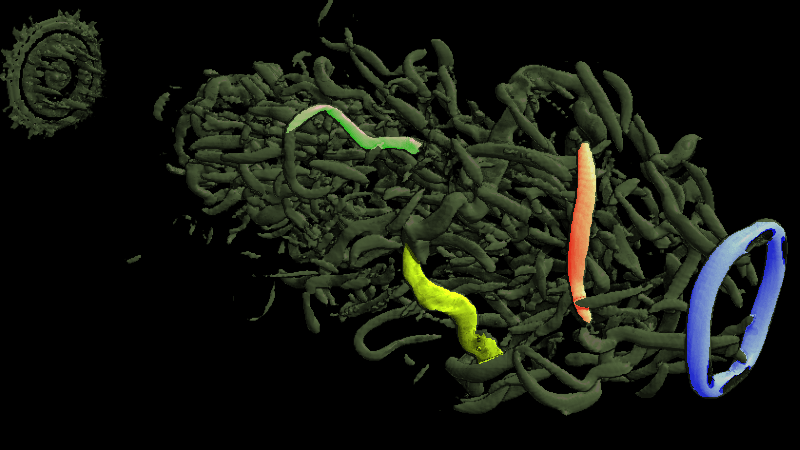
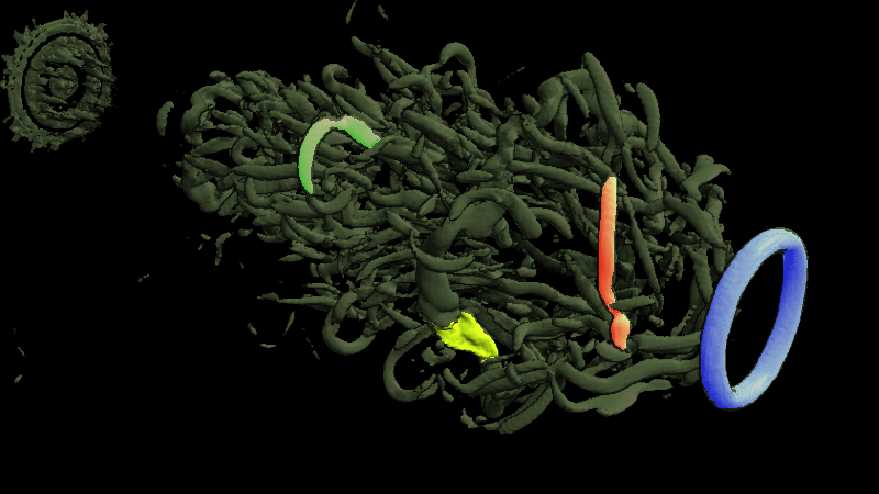
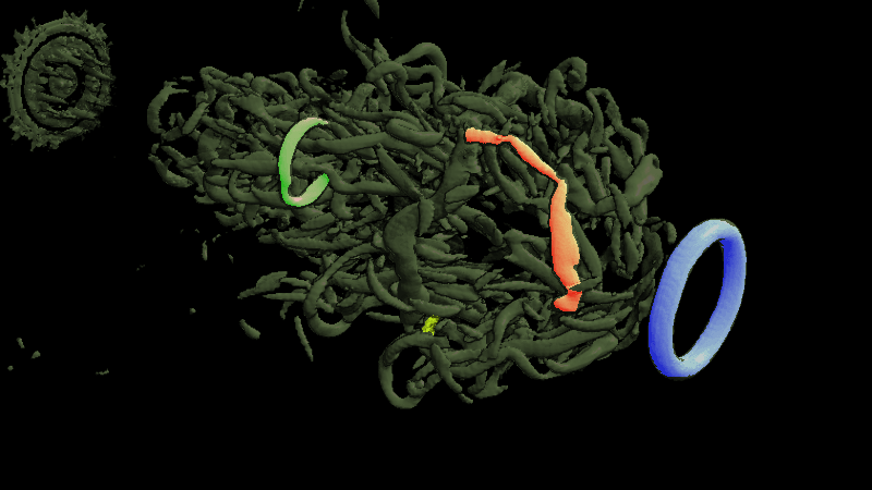
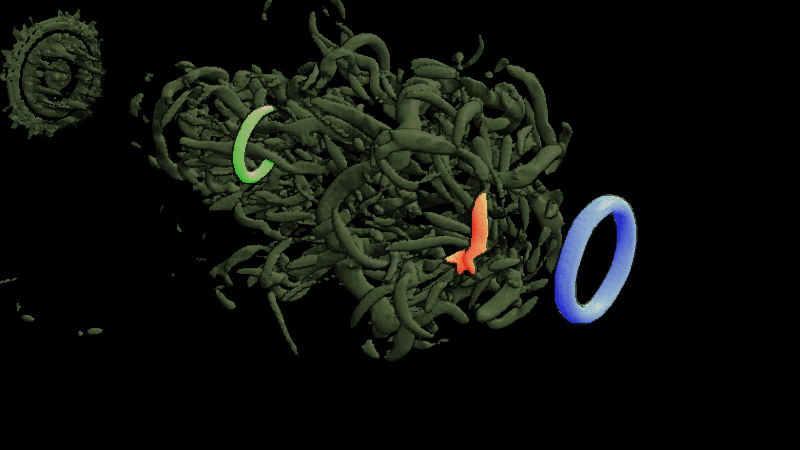
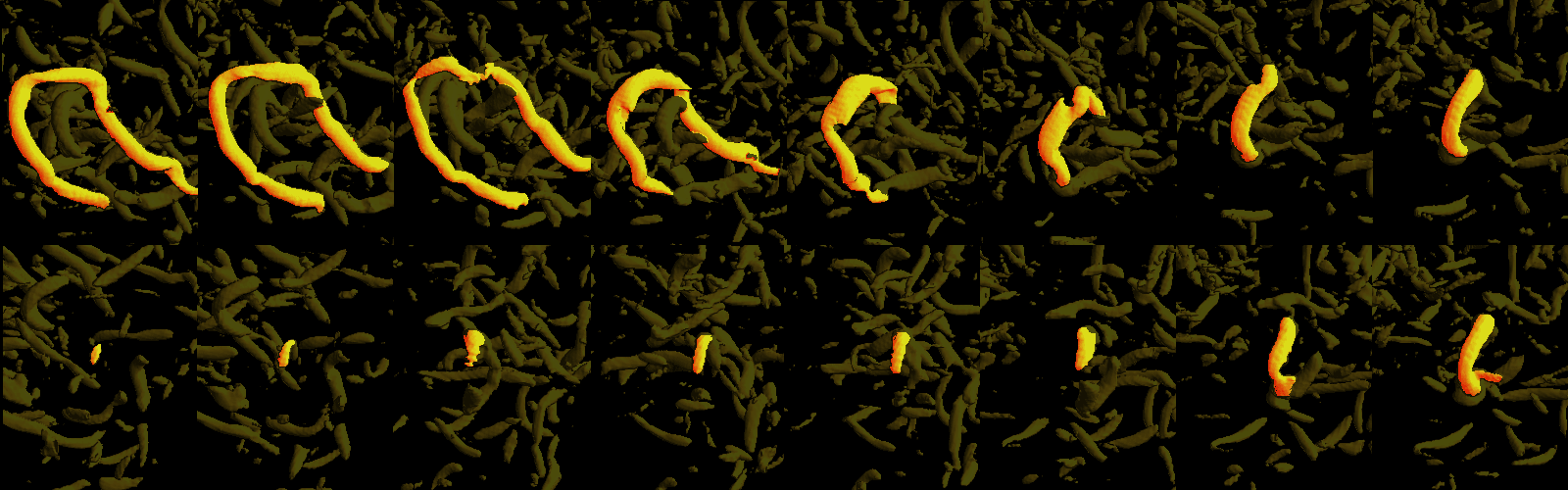
Feature Extraction and Tracking June 4th
Feature extraction is done by enabling the FET mode in the viewer by pressing 'f', then clicking the left mouse button to select a feature. The current version of feature extraction only uses the 7th layer of the depth proxy images.
Feature tracking is a proof of concept at the moment.
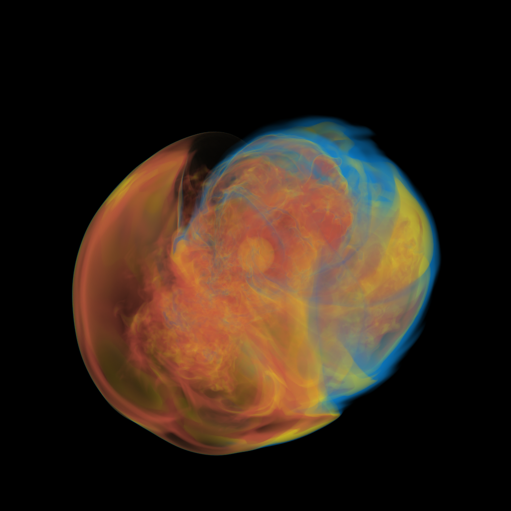
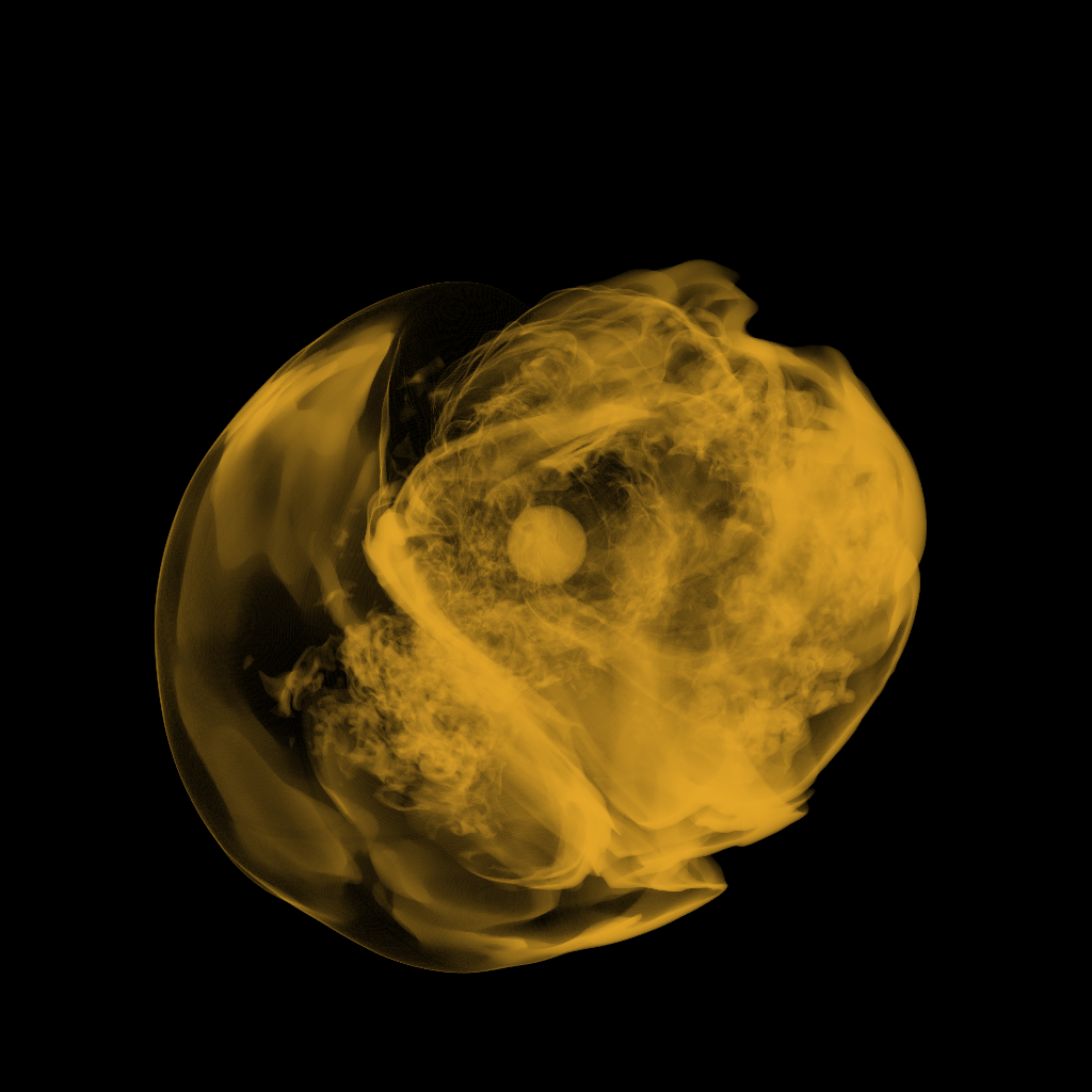
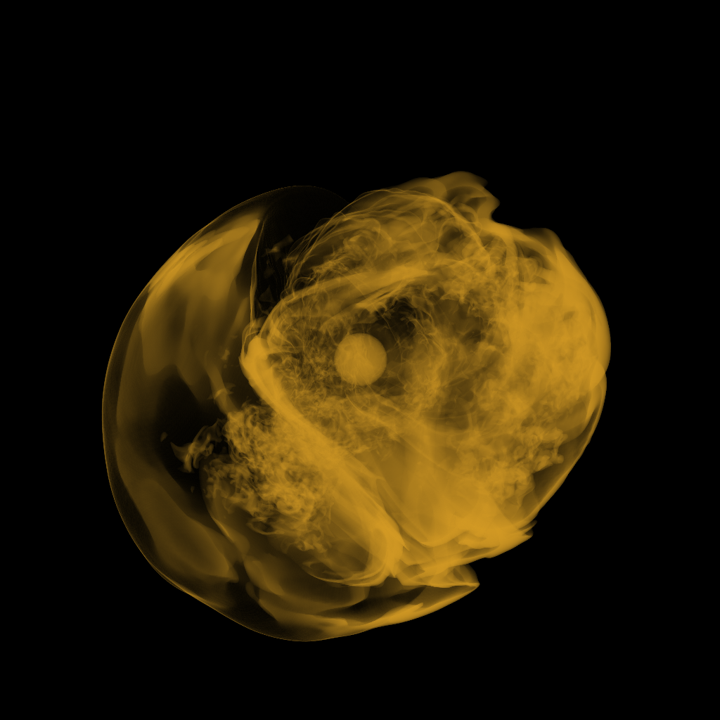
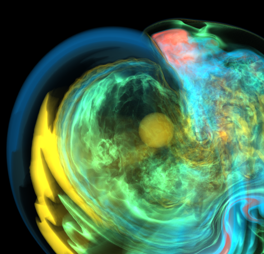
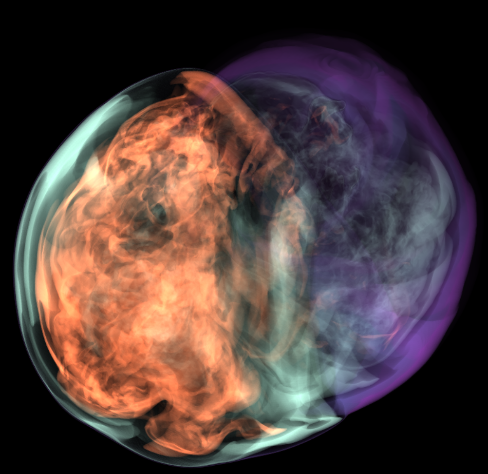
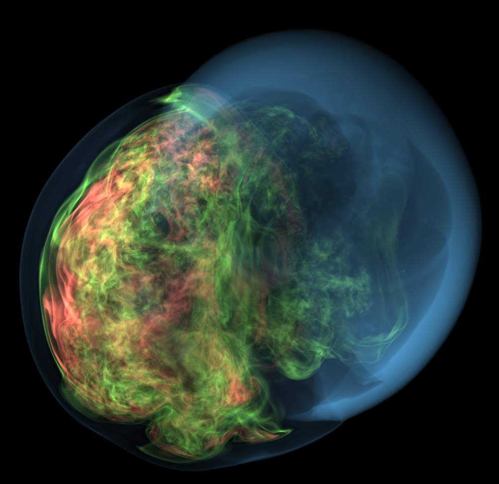
Adaptive Binning June 4th
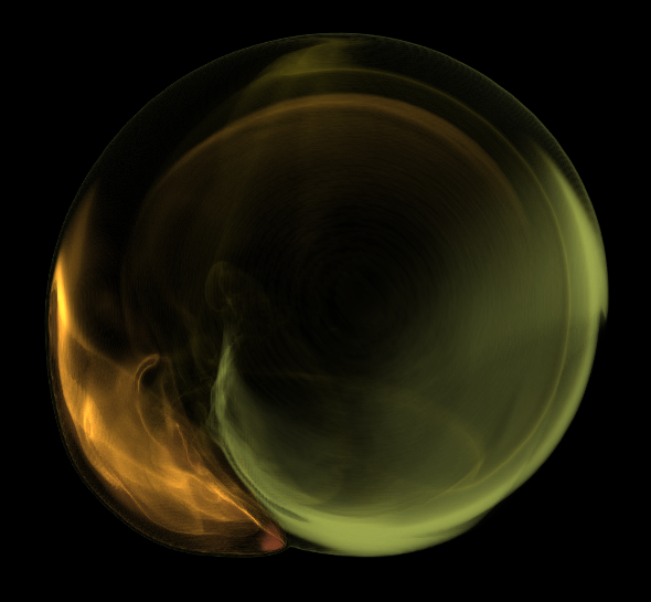
Using adaptive binning, we are able to reveal more layers in the interesting regions of the supernova dataset. Note that these images are rendered without lighting.
Because of the complex features in supernova, adding lighting is non trivial. For a single isovalue, the depth proxy image generated only shows the first layer of the isosurface. However, the isosurfaces in the supernova are like manifolds, which they wrap around multiple times. As a result, using a single layer of depth proxy image to approximate the normal map for such isosurface is wrong.
The last two images are generated using Dr. Ono's simulation. We can change the binning range to match the data distribution in the intensity domain so that more features can be shown.
All Possible Features in Supernova May 25th
By using the simplified default transfer function technique, these are the all possible isosurfaces that can be generated with the supernova dataset. Not much internal features are visualized.
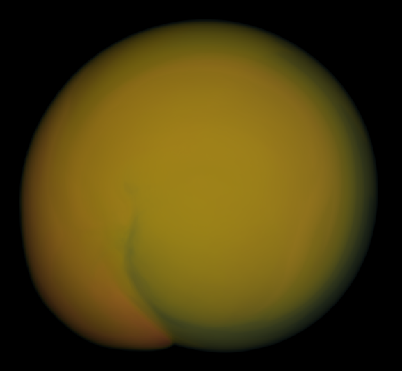
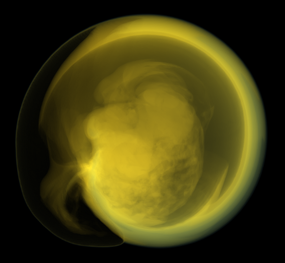
First Image from In Situ May 17th
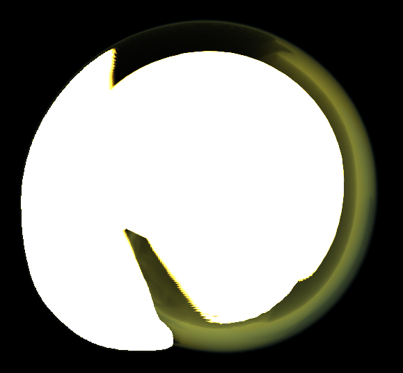
These two images are explorable images generated in situ with Dr. Ono's simulation. This is the beginning of the simulation so only a small ring is visible at the entrance. The difference is that the first image is generated from a single process and the second image is generated using MPI with 8 processes.
The problem now is Dr. Ono's simulation order the domains differently than Hongfeng's parallel renderer, so I will need to figure out how to change the composition order. That is why the second image breaks the ring into four corners.
Probably the Final Revision of the Rendering Side May 9th
I fixed most of the artifacts, both from rendering and compositing. I changed the rendering equation slightly to accomodate to the depth buffers. The concept is to render isosurfaces instead of volume rendering according to the given transfer function. The reason is people tend to create small slabs in the opacity map to create these thin semi-transparent isosurfaces.
In terms of coding, it's actually a very small change from the previous revision. Now I am only testing if a ray segment cross the average value of a bin and attenuate if it does. Also, the attenuation is fixed to 1/16 if a ray segment cross the average value of a bin. It's sort of cheating, but we can argue that it looks better and the user doesn't need to provide a transfer function anymore.
Next I will be generating results using this revision. I will generate 2 sets, 1 with supernova and 1 with Dr. Ono's simulation. Then I will start writing the paper. Bob will work on the smoother normal implementation and then the interface to select feature. Yang, well, will continue to work on the feature tracking.
Simple Integration over Ray Segments May 8th
I implemented "preintegration" like feature. When a ray segment cross multiple bins, it should add the attenuation to each of the bins instead of the bin at the end of the ray segment. And of course the boundary artifacts come back for no reason...
Image 1: without "preintegration," Image 2: with "preintegration." The iso surfaces look alot better. Image 3: with depth. We can see the boundary artifacts again.
Bob is working on smoothing the normals.
Yang is working on tracking the features. He have a set of RAF files of Dr. Ono's simulation to work with.
Current Stage of Depths/Normals and Viewer May 4th
As Kwan-Liu pointed out, the images generated with MPI don't have lighting, so I was trying to fix it. The reason happens to be that the depth values are initialized to 0 for rays that are not intersecting the bounding box. As a result, when we composite the images from different processors, we use the smallest depth value, which is 0. It's fixed now, but there are other problems with depth.
I tried to compute depth with different intensity values. Image 1 is using the lowest intensity value of a bin and image 2 is using the average intensity of a bin. They don't differentiate much. I think we need a better method to compute the depth/normal so that we don't have those black lines.
We extracted the viewer from the original messy one. The current one is more robust and allows resizing the window. Bob will continue on extending this viewer to allow temporal exploration.
Boundary Artifacts Conquered May 1st
I found the bug. It is a small but serious bug in the attenuation calculation. It was using
accumulate_alpha += current_alpha
and then clamp the accumulate_alpha to [0, 1], which is wrong but the image generated looked ok. After changing it to
Image 1 is using the correct equation. Image 2 is using the wrong equation but not clamp to [0, 1]. Image 3 is using the wrong equation and clamp to [0, 1].
Found Some Artifacts at Boundary May 1st
I was trying to clean the codes and make it run in a cluster (thehead). When I make it to run in parallel, I found some artifacts at the process boundaries. As shown in image 2 and image 3.
It seems that these artifacts only appears when we are generating RAF formats because image 1 (a static image) does not have the artifacts.
There is a function named "block_exchange_boundary()" in Hongfeng's codes. It is used to exchange boundary volume data and it fixed the boundary artifacts when we are generating static images. However, the situation is different when we are generating RAF images. If we enable "block_exchange_boundary()", it generates image 2. If we do not enable "block_exchange_boundary()", it generates image 3. That is, it fixes some of the artifacts.
Smoother Supernova Video April 28
There are two jumps in the video:
At 1/4 of the video: That is caused by 2 missing frames. I tried to smooth it out by editting the video. The video you are seeing now is the smoothed version.
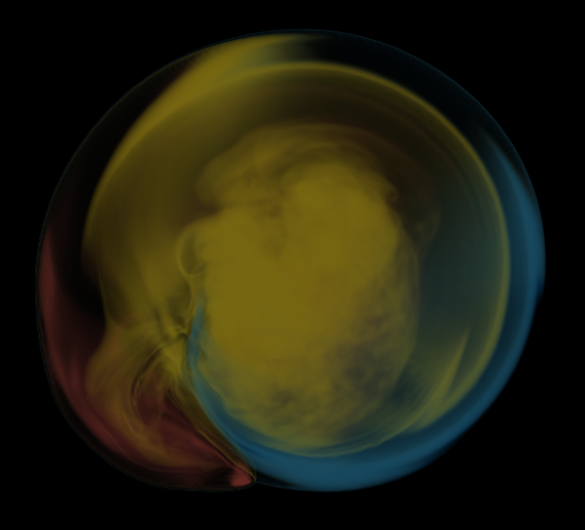
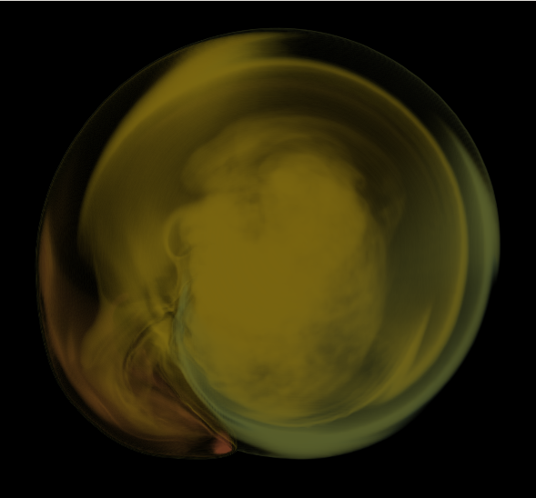
About 1/2 of the video, where the core of the supernova suddenly becomes solid. Two reasons: 1) The data actually is moving very fast at that moment. Better temporal resolution? 2) My guess is a huge chunk of data crossed boundary of the intensity bins at that moment, which turns a lot of yellow into green.
The First Supernova Video April 27
Combined the images of supernova into a video. There are some jumps in the video. Two reasons: 1) The supernova dataset is missing 2 timesteps of data (1461 and 1462). 2) There were 4 timesteps that were unable to render for unknown reason. (1466, 1467, 1564 and 1565).
Fixed Normals April 27
I fixed an issue in the normal estimation process based on Bob's input. Images from left to right are from timestep 1403, 1440, 1470, 1540 and 1580. A few things:
There are still visible artifacts (the black lines). Those are where the depth layers disjoint. We might be able to interpolate a more accurate depth value based on neighbor bins, but I don't think I can make the fix in time.
It was my mistake that used a viewport that only captures the first timestep entirely. It seems like the supernova moves around significantly.
Using one transfer function is not enough for the whole time span of this supernova dataset. When the transfer function looks good in 1580, it doesn't look interesting in 1403. That actually makes it more interesting because we can demonstrate how explorable images can deal with this problem.
Need Input for Transfer Function April 26
This image is generated using the transfer function on the left, also I hard coded it to cutaway the front part. There are artifacts which I do not understand why/how. I assume they are artifacts from the viewing stage. Generating such an image is time consuming, generating a image sequence can take hours, so we have 1 chance (tonight) to generate the video.
As long as the view angle and the opacity map is good enougth, we can change the colors later. And I hope I can fix the artifacts tomorrow.
Bob, do you have any idea where these artifacts might come from?
Video from Dr. Ono's Simulation Data April 26
This is actually generated using ParaView. It is intended to be used by Yang to make a proof of concept video for feature tracking because making the actual feature tracking to work is time consuming and we don't have enough time at this stage.
Lighting with Depth Proxy April 25
From Bob:
I've added Phong lighting to Chris's viewer (Actually I was done with that at about 9PM).
What I've been experimenting with since then is: I don't understand the behavior I'm getting from the transfer function editor. I believe it's what Chris is complaining about with respect to the assumptions made within the structure of the RAFs. Color modulation works great, but opacity modulation is extremely finicky: If I even slightly raise the low intensity value opacity, the higher values are either completely hidden or oversaturate immediately. I confirmed that Chris's code conforms to the description in the paper, so there must be something Anna and the others felt to be trivial that's necessary to fix it. Chris: I think we can fix this issue now that we have the depths, by sorting the bins by depth before rendering. I'm tired for now, but I'll test my hypothesis tomorrow. My implementation is on our dropbox share.
The first attached image is just a quick demonstration with opacity disabled so that you can more clearly see the lighting changes. It's just the Phong model: The parameters are all configurable within the shader, and whenever we like we can expose them in the interface.
The second attached image is the same except with opacity enabled. I recognize the quality is bad: as I said, I really had to play around a lot with the opacities to get a half-decent picture...this needs to be fixed, so hopefully my idea will work.
Wrong Lighting April 20
As Hongfeng recommended, I used amb_diff as attenuation in the ray attenuation function, which is mathematically incorrect. Because by using amb_diff, we actually revealed the bins that should be occluded.
For example, we have slab A and slab B, where slab A is in front of slab B and slab A is fully opaque. If we are using alpha as attenuation, we will not be able to see slab B, which is correct, but if we use amb_diff as attenuation, we will be seeing slab B because slab A is no longer fully opaque.
First Image from Dr. Ono's Simulation April 18
This image is rendered from Dr. Ono's simulation output data. This is not genereated in situ, rather I used the output data that Yang generated in the past. And this is not generated in parallel because the data is not stored in a parallel way.
Opacity Modulation April 18
Implemented opacity modulation as described in the paper. The 3 images are generated from a single explorable image.
We can change the opacity map to reveal internal structures, from image 1 to image 2.
They made a big assumption that a ray traverse from low intensity to high intensity. As a result, when we change the opacity value of a lower intensity bin, it affects the opacity of the higher intensity bins. In image 3, we lower the opacity value of some lower intensity bins, it amplifies the opacity values in the higher intensity bins, which makes them all white.
Rendered with Smaller Step Size April 18
These images are rendered with a ray step size 0.5, which eliminates the ring artifacts. Of course we can change the colors. I tried to incorporate opacity change in the third image. This opacity change doesn't have opacity modulation. I am going to implement it next.
First Images April 17
This is the first sets of explorable images generated using Hongfeng's codes. They are generated using a fairly big ray step size (2.0). That is why the ring like artifacts appear. I am using a big step size because it is slow since it is a software renderer. The two images demonstrate that we can change the colormap, but I still need to add the functonality in the viewer to be able to change the opaicty map.